Aplicativo web para el control administrativo y seguimiento del progreso físico de los clientes del gimnasio Vital GYM.
Actualmente el gimnasio Vital GYM no dispone de ningún software o aplicativo web enfocado al control administrativo y al seguimiento físico de usuarios, todo se lo lleva de una manera rudimentaria, es decir mediante el uso de lápiz y papel, y por ende esto hace mucho más difícil el trabajo para el personal encargado.
Una gran parte de personas, en busca de cuidar su salud y su apariencia acuden regularmente a gimnasios tratando de encontrar ayuda profesional, por esta razón el mercado actual ha creado este tipo de negocios en la ciudad de Quito, los mismos que tratan de ofrecer los mejores precios y servicios al cliente, pero la gran mayoría de gimnasios no cuentan con ningún tipo de aplicativo, que gestione correctamente todos los procesos y las tareas comunes que se hacen día a día en los mismos. Es por esto que se genera la necesidad de crear un aplicativo que administre y automatice las actividades de gimnasios.
Este será accesible desde cualquier computador, estará disponible las 24 horas del día los 365 días del año, a través de internet y su propio servidor. Esto es una gran ventaja, tanto para el propietario como para clientes e instructores del gimnasio. Todos estos podrán acceder al aplicativo desde cualquier lugar y la hora que deseen, para Consultar pagos, asistencia y su progreso. El aplicativo será accesible desde tablets, smartphones, ipads, smarts TV etc. ya que el mismo de adaptará a cualquier tamaño de pantalla o resolución.
Vulnerabilidades de Seguridad
Si descubre una vulnerabilidad de seguridad dentro de este software, envía un correo electrónico a Soporte a support@vitalgymecuador.com Todas las vulnerabilidades de seguridad serán tratadas los más rápido posible.
Licencia
Vital Gym es un software de código abierto bajo licencia MIT license. Desarrollado bajo el Framework Laravel
Robofinder is a powerful Python script designed to search for and retrieve historical robots.txt files from Archive.org for any given website. This tool is ideal for security researchers, web archivists, and penetration testers to uncover previously accessible paths or directories that were listed in a site’s robots.txt.
Features
Fetch historical robots.txt files from Archive.org.
Extract and display old paths or directories that were once disallowed or listed.
Save results to a specified output file.
Silent Mode for unobtrusive execution.
Multi-threading support for faster processing.
Option to concatenate extracted paths with the base URL for easy access.
Debug mode for detailed execution logs.
Extract old parameters from robots.txt files.
Installation
Using pipx
Install Robofinder quickly and securely using pipx:
Contributions are highly welcome! If you have ideas for new features, optimizations, or bug fixes, feel free to submit a Pull Request or open an issue on the GitHub repository.
txtnish is a client for twtxt–the
decentralised, minimalist microblogging service for hackers.
Instead of signing up at a closed and/or regulated microblogging platform,
getting your status updates out with twtxt is as easy as putting them in a
publicly accessible text file. The URL pointing to this file is your identity,
your account. twtxt then tracks these text files, like a feedreader, and builds
your unique timeline out of them, depending on which files you track. The
format is simple, human readable, and integrates well with UNIX command line
utilities.
All subcommands of txtnish provide extensive help, so don’t hesitate
to call them with the -h option.
If you are a new user, there is a quickstart command that will ask you some
questions and write a configuration file for you:
$ txtnish quickstart
Installation
txtnish only depends on tools you normally find in a POSIX environment: awk, sort, cut and sh. There are only two exceptions: you need curl
to download twtxt files and a xargs that support parallel processing
via -P. You can use a xargs without, but then txtnish falls back to
downloading one url after another.
Installation itself is as easy as it gets: just copy the script somewhere
in your PATH.
Subcommands
tweet
Appends a new tweet to your twtxt file. There are three different ways
to input tweets. You can either pipe them into tweet, or pass them along
as arguments. When you call txtnish tweet without any arguments and
it’s not connected to a pipe, it will call $EDITOR for you and tweet
any line as a separate tweet.
timeline
Retrieves your personal timeline.
publish
Publishes your twtfile. This is especially helpful after you changed your post_tweet_hook.
follow
Adds a new source to your followings.
unfollow
Removes an existing source from your followings.
following
Prints the list of the sources you’re following.
reply
Displays an outcommented version of your timeline in $EDITOR. Every
line that is not commented after you saved and exited the editor, will
be tweeted.
Search tweets
You can provide a search expression to filter your timeline with the flag -S. The search expression is an awk conditional with four predefined
variables:
At startup txtnish checks whether ~/.config/txtnish/config exists and
will source it if it exists. The configuration file must be a valid
shell script.
General
add_metadata
Add metadata to twtxt file. Default to 0 (false).
awk
Path to the awk binary. Defaults to awk.
sed
Path to the sed binary. Defaults to sed.
limit
How many tweets should be shown in timeline. Defaults to 20.
formatter
Defined which command is used to wrap each tweet to fit on the screen. It
defaults to fold -s.
sort_order
How to sort tweets. This option can be either ascending or descending. ascending prints the oldest tweet first, descending the
newest. This value can be overridden with the -d and -a flags.
timeout
Maximum time in seconds that each http connection can take. Defaults
to zero.
use_color
If the output should be colorized with ANSI escape sequences. See the
section COLORS on how to change the color settings. Defaults to 1.
pager
Which pager to use if use_pager is enabled. Default to less -R in order
to display colors. This can be toggled with -p or -P to enable or
disable the pager. Defaults to 1.
disclose_identity
If set to 1, send your nick and twturl with every http request. This
makes only sense if you also set twturl and nick. Defaults to 0.
nick
Your nick. This is used to collapse mentions of your twturl and is send to
all feeds you’re following if disclose_identity is set to 1.
Defaults to the environment variable $USER.
twturl
The url of your feeds. This is used to collapse mentions and is send to
all feeds you’re following if disclose_identity is set to 1. Defaults
to the environment variable $USER.
always_update
Always update all feeds before showing tweets. If you set this variable
to 0, you need to update manually with the update command.
http_proxy
Sets the proxy server to use for HTTP.
https_proxy
Sets the proxy server to use for HTTPS.
sign_twtfile
If set to 1, sign the twtfile with pgp. Defaults to 0.
In case you are also overwriting the post_tweet_hook note that this
will create a signed file in a temporary directory and change the value of twtfile accordingly. Your twtfile will not be changed!
Signing your twtfile might break some twtxt clients as lines without
a TAB are not allowed by a strict reading of the spec.
check_signature
Verify pgp signatures and show the result in the timeline if set to 1. Defaults to 0.
sign_user
Sets a different local user to sign twtfile than what is the default. It will
print a message indicating an override is in place.
gpg_bin
Sets custom name of gpg executable.
ipfs_gateway
When you subscribe to an ipns:// address, txtnish will call this gateway to get
the users twtfile. Defaults to http://localhost:8080 and falls back to https://ipfs.io if txtnish can’t reach the gateway.
Publish with scp
scp_user
Use the given username to connect to the remote server. Required to publish
with scp.
scp_host
Copy twtfile to this host. Required to publish with scp.
scp_remote_name
Name of twtfile on remote host. Defaults to the basename of the twtfile.
sftp_over_scp
Use SFTP instead of SCP if set to 1.
Publish with ftp
ftp_user
Use the given username to connect to the remote server. Required to publish
with ftp.
ftp_host
Copy twtfile to this host. Required to publish with ftp.
ftp_remote_name
Name of twtfile on remote host. Defaults to the basename of the twtfile.
Publish with IPFS
ipfs_publish
Publish the twtfile with ipfs if set to 1. Defaults to 0.
You will need the ipfs tools and a running daemon to publish to ipfs.
ipfs_wrap_with_dir
Call ipfs add with --wrap-with-dir if set to 1. Defaults to 0.
ipfs_recursive
Call ipfs add with --recursive if set to 1. The complete directory of
your twtfile will be published. Defaults to 0.
Colors
If use_color is set to 1, the nick, timestamp, mentions and hashtags
will be colorized. txtnish recognizes black, red, green, yellow, blue,
magenta, cyan and white. You can set the background color with the prefix on_.
color_nick="yellow on_white"
Additional a color definiation can specify the attributes bold, bright,
faint, italic, underline, blink and fastblink if your terminal supports
them.
color_nick="yellow on_white blink"
The order of colors and attributes doesn’t matter and multiple attributes can
be combined.
To customize the behaviour of txtnish the user can override functions.
pre_tweet_hook
This hook is called before a new tweet is appended to your twtfile. This can be
useful if you’re using txtnish on multiple devices and want to update your
local twtfile before appending to it. There’s a predefined function sync_twtfile that does exactly that.
pre_tweet_hook () {
	sync_twtfile
}
post_tweet_hook
post_tweet_hook is called after txtnish has appended new tweets to your
twtfile. It’s a good place to uploade your file somewhere.
This program is free software: you can redistribute it and/or modify it under
the terms of the GNU General Public License as published by the Free Software
Foundation, either version 3 of the License, or (at your option) any later
version.
This program is distributed in the hope that it will be useful, but WITHOUT ANY
WARRANTY; without even the implied warranty of MERCHANTABILITY or FITNESS FOR A
PARTICULAR PURPOSE. See the GNU General Public License for more details.
You should have received a copy of the GNU General Public License along with
this program. If not, see http://www.gnu.org/licenses/.
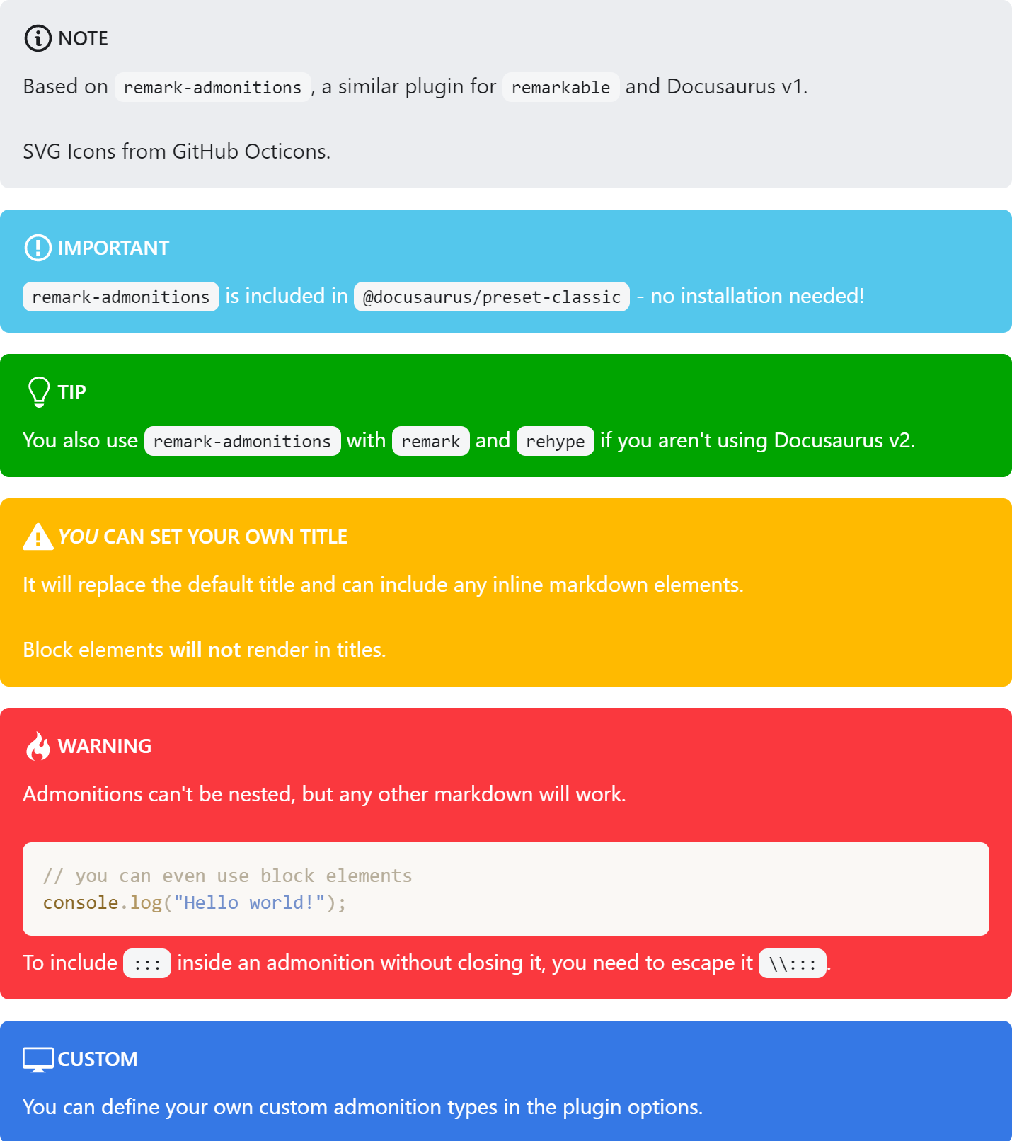
A remark plugin for admonitions designed with Docusaurus v2 in mind.
remark-admonitions is now included out-of-the-box with @docusaurus/preset-classic!
Installation
remark-admonitions is available on NPM.
npm install remark-admonitions
unified + remark
If you’re using unified/remark, just pass the plugin to use()
For example, this will compile input.md into output.html using remark, rehype, and remark-admonitions.
constunified=require('unified')constmarkdown=require('remark-parse')// require the pluginconstadmonitions=require('remark-admonitions')constremark2rehype=require('remark-rehype')constdoc=require('rehype-document')constformat=require('rehype-format')consthtml=require('rehype-stringify')constvfile=require('to-vfile')constreport=require('vfile-reporter')constoptions={}unified().use(markdown)// add it to unified.use(admonitions,options).use(remark2rehype).use(doc).use(format).use(html).process(vfile.readSync('./input.md'),(error,result)=>{console.error(report(error||result))if(result){result.basename="output.html"vfile.writeSync(result)}})
Docusaurus v2
@docusaurus/preset-classic includes remark-admonitions.
If you aren’t using @docusaurus/preset-classic, remark-admonitions can still be used through passing a remark plugin to MDX.
Usage
Admonitions are a block element.
The titles can include inline markdown and the body can include any block markdown except another admonition.
The general syntax is
:::keyword optional title
some content
:::
For example,
:::tip pro tip
`remark-admonitions` is pretty great!
:::
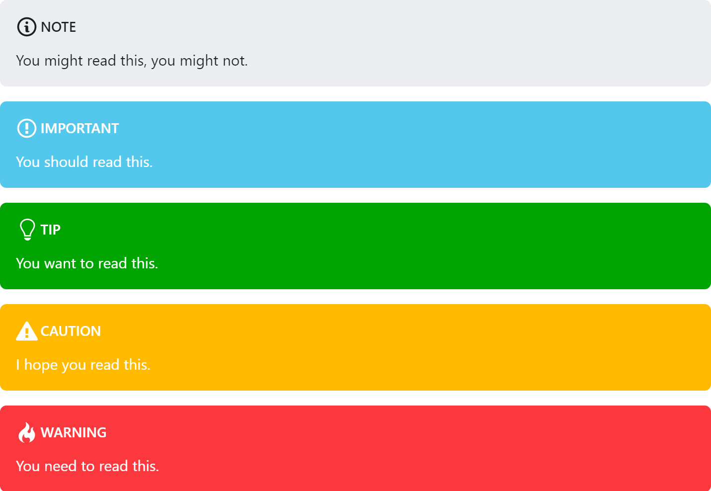
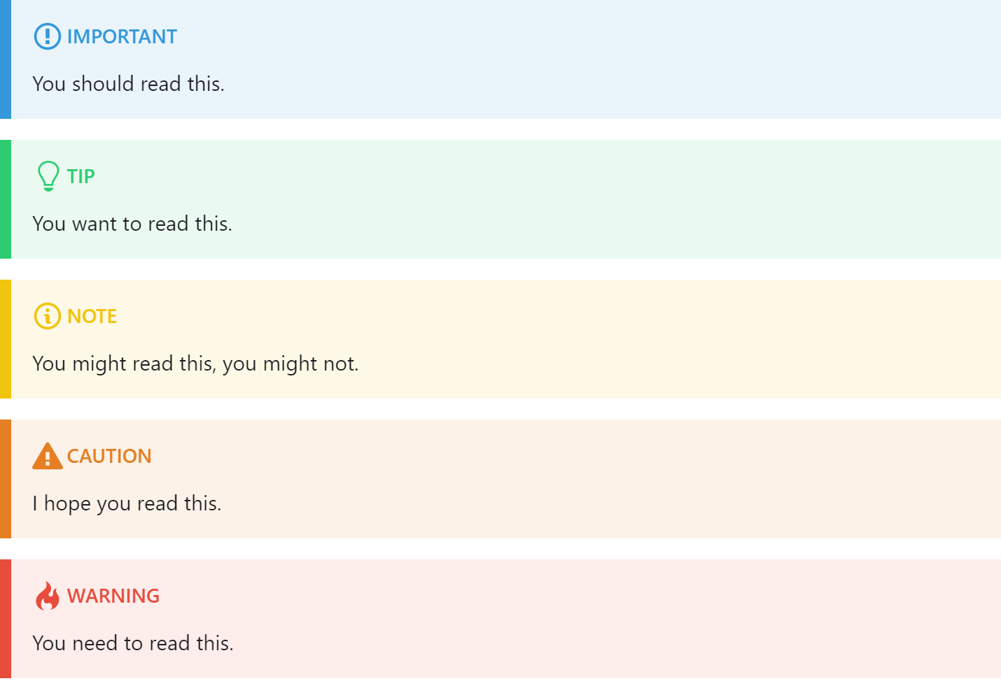
The default keywords are important, tip, note, warning, and danger.
Aliases for info => important, success => tip, secondary => note and danger => warning have been added for Infima compatibility.
Options
The plugin can be configured through the options object.
Defaults
constoptions={customTypes: customTypes,// additional types of admonitionstag: string,// the tag to be used for creating admonitions (default ":::")icons: "svg"|"emoji"|"none",// the type of icons to use (default "svg")infima: boolean,// wether the classes for infima alerts should be added to the markup}
Custom Types
The customTypes option can be used to add additional types of admonitions. You can set the svg and emoji icons as well as the keyword. You only have to include the svg/emoji fields if you are using them.
The ifmClass is only necessary if the infima setting is true and the admonition should use the look of an existing Infima alert class.
We believe in a future in which the web is a preferred environment for numerical computation. To help realize this future, we’ve built stdlib. stdlib is a standard library, with an emphasis on numerical and scientific computation, written in JavaScript (and C) for execution in browsers and in Node.js.
The library is fully decomposable, being architected in such a way that you can swap out and mix and match APIs and functionality to cater to your exact preferences and use cases.
When you use stdlib, you can be absolutely certain that you are using the most thorough, rigorous, well-written, studied, documented, tested, measured, and high-quality code out there.
To join us in bringing numerical computing to the web, get started by checking us out on GitHub, and please consider financially supporting stdlib. We greatly appreciate your continued support!
spttrf
Compute the L * D * L^T factorization of a real symmetric positive definite tridiagonal matrix A.
Installation
npm install @stdlib/lapack-base-spttrf
Alternatively,
To load the package in a website via a script tag without installation and bundlers, use the ES Module available on the esm branch (see README).
If you are using Deno, visit the deno branch (see README for usage intructions).
The branches.md file summarizes the available branches and displays a diagram illustrating their relationships.
To view installation and usage instructions specific to each branch build, be sure to explicitly navigate to the respective README files on each branch, as linked to above.
Usage
varspttrf=require('@stdlib/lapack-base-spttrf');
spttrf( N, D, E )
Computes the L * D * L^T factorization of a real symmetric positive definite tridiagonal matrix A.
varFloat32Array=require('@stdlib/array-float32');varD=newFloat32Array([4.0,5.0,6.0]);varE=newFloat32Array([1.0,2.0]);spttrf(3,D,E);// D => <Float32Array>[ 4, 4.75, ~5.15789 ]// E => <Float32Array>[ 0.25, ~0.4210 ]
The function has the following parameters:
N: order of matrix A.
D: the N diagonal elements of A as a Float32Array.
E: the N-1 subdiagonal elements of A as a Float32Array.
Note that indexing is relative to the first index. To introduce an offset, use typed array views.
spttrf.ndarray( N, D, strideD, offsetD, E, strideE, offsetE )
Computes the L * D * L^T factorization of a real symmetric positive definite tridiagonal matrix A using alternative indexing semantics.
varFloat32Array=require('@stdlib/array-float32');varD=newFloat32Array([4.0,5.0,6.0]);varE=newFloat32Array([1.0,2.0]);spttrf.ndarray(3,D,1,0,E,1,0);// D => <Float32Array>[ 4, 4.75, ~5.15789 ]// E => <Float32Array>[ 0.25, ~0.4210 ]
The function has the following additional parameters:
strideD: stride length for D.
offsetD: starting index for D.
strideE: stride length for E.
offsetE: starting index for E.
While typed array views mandate a view offset based on the underlying buffer, the offset parameters support indexing semantics based on starting indices. For example,
varFloat32Array=require('@stdlib/array-float32');varD=newFloat32Array([0.0,4.0,5.0,6.0]);varE=newFloat32Array([0.0,1.0,2.0]);spttrf.ndarray(3,D,1,1,E,1,1);// D => <Float32Array>[ 0.0, 4.0, 4.75, ~5.15789 ]// E => <Float32Array>[ 0.0, 0.25, ~0.4210 ]
Notes
Both functions mutate the input arrays D and E.
Both functions return a status code indicating success or failure. A status code indicates the following conditions:
0: factorization was successful.
<0: the k-th argument had an illegal value, where -k equals the status code value.
0 < k < N: the leading principal minor of order k is not positive and factorization could not be completed, where k equals the status code value.
N: the leading principal minor of order N is not positive, and factorization was completed.
spttrf() corresponds to the LAPACK routine spttrf.
Examples
vardiscreteUniform=require('@stdlib/random-array-discrete-uniform');varspttrf=require('@stdlib/lapack-base-spttrf');varopts={'dtype': 'float32'};varD=discreteUniform(5,1,5,opts);console.log(D);varE=discreteUniform(D.length-1,1,5,opts);console.log(E);// Perform the `L * D * L^T` factorization:varinfo=spttrf(D.length,D,E);console.log(D);console.log(E);console.log(info);
C APIs
Usage
TODO
TODO
TODO.
TODO
TODO
TODO
Examples
TODO
Notice
This package is part of stdlib, a standard library for JavaScript and Node.js, with an emphasis on numerical and scientific computing. The library provides a collection of robust, high performance libraries for mathematics, statistics, streams, utilities, and more.
For more information on the project, filing bug reports and feature requests, and guidance on how to develop stdlib, see the main project repository.
ACM TOMS Algorithm 905: SHEPPACK: Modified Shepard Algorithm for Interpolation of Scattered Multivariate Data
SHEPPACK is a Fortran 95 package containing five versions of the modified Shepard algorithm: quadratic (Fortran 95 translations of Algorithms 660, 661, and 798), cubic (Fortran 95 translation of Algorithm 791), and linear variations of the original Shepard algorithm. An option to the linear Shepard code is a statistically robust fit, intended to be used when the data is known to contain outliers. SHEPPACK also includes a hybrid robust piecewise linear estimation algorithm RIPPLE (residual initiated polynomial-time piecewise linear estimation) intended for data from piecewise linear functions in arbitrary dimension m. The main goal of SHEPPACK is to provide users with a single consistent package containing most existing polynomial variations of Shepard’s algorithm. The algorithms target data of different dimensions. The linear Shepard algorithm, robust linear Shepard algorithm, and RIPPLE are the only algorithms in the package that are applicable to arbitrary dimensional data.
This code has been re-uploaded with the permission of Drs. William Thacker
and Layne Watson.
All comments and questions should be directed to them (see contact info at
the bottom of this file).
Organizational Details
The original source code, exactly as distributed by ACM TOMS, is included in
the src directory.
The src directory also contains its own README and build instructions.
Comments at the top of each subroutine document their proper usage.
Several minor modifications to the contents of src have been made:
The included Makefile has been slightly modified to run all tests
when the make all command is run
All file extensions have been changed form .f95 to .f90 for
compiler compatibility reasons.
Reference and Contact
To cite this work, use:
    @article{alg905,
        author = {Thacker, William I. and Zhang, Jingwei and Watson, Layne T. and Birch, Jeffrey B. and Iyer, Manjula A. and Berry, Michael W.},
        title = {{Algorithm 905: SHEPPACK}: Modified {S}hepard Algorithm for Interpolation of Scattered Multivariate Data},
        year = {2010},
        volume = {37},
        number = {3},
        journal = {ACM Trans. Math. Softw.},
        articleno = {34},
        numpages = {20},
        doi = {10.1145/1824801.1824812}
    }
Inquiries should be directed to
William I. Thacker,
Department of Computer Science, Winthrop University,
Rock Hill, SC 29733; wthacker@winthrop.edu
Layne T. Watson,
Department of Computer Science, VPI&SU,
Blacksburg, VA 24061-0106;
(540) 231-7540; ltw@vt.edu
The XmlExtractor is a class that will parse XML very efficiently with the XMLReader object and produce an object (or array) for every item desired. This class can be used to read very large (read GB) XML files
$rootTags Specify how deep to go into the structure before extracting objects. Examples are below
$filename Path to the XML file you want to parse. This is optional as you can pass an XML string with loadXml() method
$returnArray If true, every iteration will return items as an associative array. Default is false
$mergeAttributes If true, any attributes on extracted tags will be included in the returned record as additional tags. Examples below
Methods
XmlExtractor.loadXml($xml)
Loads XML structure from a php string
XmlExtractor.getRootTags()
This will return the skipped root tags as objects as soon as they are available
XmlItem.export($mergeAttributes = false)
Convert this XML record into an array. If $mergeAttributes is true, any attributes are merged into the array returned
XmlItem.getAttribute($name)
Returns the record’s named attribute
XmlItem.getAttributes()
Returns this record’s attributes if any
XmlItem.mergeAttributes($unsetAttributes = false)
Merges the record’s attributes with the rest of the tags so they are accessible as regular tags. If unsetAttributes is true, the internal attribute object will be removed
The first constructor argument is a slash separated tag list that communicates to XmlExtractor that you want to extract “person” records (last tag entry) from earth -> people structure.
The export method on the $person object returns it in array form, which will look like this:
There are a number of things going on with the above XML.
The two root tags that we have to skip to get to our items have information attached.
We can get at these with the getRootTags() method. The next issue is that both items are using attributes to define their data.
This example is a bit contrived, but it will show the functionality behind the mergeAttributes feature.
By the end of this example, we will have two items with identical structure.
Once “compressed” (exported with merged attributes) the structure of both items is the same.
In the event of an attribute having the same name as the tag, the tag takes precedence and is never overwritten.
The two items will end up looking like this:
Reflections on NY Phil — The NY Phil as a lens on changes in US society
html_document
Around the turn of the century, New York City became the arts center of the world. Its establishment not only encouraged the flourishing of American musicians but also attracted musicians from all over the world to NYC. NY Philharmonic as an important art and culture institution, reflects the social and economic changes of the United States society over time. In this study I focus on NY Philharmonic data from three perspectives: 1. the nationality of composers whose works are performed by NY Philharmonic in relation to the political enviroments of the US; 2. the status of women composers over time; 3. the elasticity of an art and culture institute’s reaction to social issues by comparing NY Phil performance data and MoMA exhibition data.
The following graph shows that most of the composers’ works got performed fewer than ten times, and only 16 composers’ works are performed more than 1000 times. Therefore, I expect the composers to be diverse.
require(mosaic)
nrow(SumComp1)
hist(SumComp1$SumComp,main="number of performance histogram",xlab="number of performance")

comp1000=subset(SumComp1,SumComp>=1000)
nrow(comp1000)
comp1000

compl1000=subset(SumComp1,SumComp<=10)
nrow(compl1000)
hist(compl1000$SumComp,main="number of performance histogram",xlab="number of performance")
According to Marx, economics base determines the superstructure of the society, which is reflected as the economic development level determines the politics, art and culture activity of a society. Originally, I was thinking of studying the relationship between the number of contemporary composers’ works performed at NY Philharmonic and the GDP growth rate to see how the number of contemporary composers work performed reflects society’s emphasis on art and music education. But the list of composers’ birth and death year is incomplete. Therefore I cannot determine which composers are alive at the time their works are performed by the NY Phil. Thus in order to see the relationship between US economic development and NY Phil performances, I decided to study the relationship between the number of concerts in each season and US GDP growth rate. The graph shows that GDP growth rate and performance don’t have similar patterns. However, from a micro perspective, the number of performance per year reflects the NY Phil’s own economic condition. For example, the boom of the number of performance at the beginning of the twentieth century is explained by recognizing that several orchestras merged.
3.Normalized Performance Frequency Score
Because the number of performance change year by year, I computed a “Normalized Performance Frequency Score” to normalize by total number of performances. I got the normalized performance frequency score by dividing the number of performances for each composers in each season by the total number of performance in each season.
require(base)
composerBySeasonComplete[is.na(composerBySeasonComplete)] <- 0
composerBySeasonComplete1=composerBySeasonComplete[2:175]
composerBySeasonComplete2=composerBySeasonComplete[1]
popScoreComposerComplete=data.frame()
totalNumConcert=colSums(composerBySeasonComplete1, na.rm=TRUE)
for ( i in 1:2652){
  popScoreComposerComplete[i,]=composerBySeasonComplete1[i,]/totalNumConcert
  i=i+1
}
popScoreComposerComplete=cbind(composerBySeasonComplete2,popScoreComposerComplete)
write.csv(popScoreComposerComplete,"popScoreComposerComplete.csv")
the Normalized Performance Frequency Score table looks like:
art and politics can affect each other. In this part, I want to ask several questions:
As NYC rise to be the center of art and culture, does the number of American composers’ works increase?
Does the number of German composers’ work decrease during WWI and WwII?
Does the number of Russian composers’ work decrease during the cold war?
As the economy rises in Asian and Latin American countries, does the number of works from these areas increase over time?
To do this we need to identify the nationality of composers whose works are performed by the NY Philharmic. The NY Philharmonic data do not have the nationalities of composers. Therefore, I scraped wikipedia page and got data on composers’ nationalities.
I got the most of the composers nationality scores by scraping this page and the links in the page: (https://en.wikipedia.org/wiki/Category:Classical_composers_by_nationality) using the following python code
####American.
I stacked the data from multiple pages, cleaned them and matched them with the normalized performance frequency score table and computed the proportion of the number of American composers whose works are performed by the NY Philharmonic over total number of works performed by the NY Philharmonic over time.
The graph shows a general increase of the proportion of the number of American composers over total number of composers over time which reinforces the hypothesis that as America rise to become the center of the art and culture of the world during the turn of the century its composers got more recognitions by the NY Philharmonic.
load("germanComps.RData")

l=c()
for ( i in 1:length(german1.3)){
  l=c(l,which(german1.3[i]==popScoreComposerComplete$composers))
}
german=popScoreComposerComplete$composers[l]
germanPop=popScoreComposerComplete[l,]
germanPopSum=colSums(germanPop[2:175])
qplot(seq_along(germanPopSum),germanPopSum)+geom_line()+ylim(0,1)+geom_area(colour="black")+scale_x_continuous(breaks=seq(1,175,10),labels=c("1842","1852","1862","1872","1882","1892","1902","1912","1922","1932","1942","1952","1962","1972","1982","1992","2002","2012"))+ theme(axis.text.x = element_text(angle = 45,size=10, hjust = 1))+xlab("seasons")+ylab("percentage of works being performed")+ggtitle("German Composers")
the graph shows a significant decrease in the proportion of German composers’ works being performed during WWI and WWII and after WWII.
wagner=as.numeric(popScoreComposerComplete[81,2:175])
qplot(seq_along(wagner),wagner)+geom_line()+ylim(0,1)+geom_area(colour="black")+scale_x_continuous(breaks=seq(1,175,10),labels=c("1842","1852","1862","1872","1882","1892","1902","1912","1922","1932","1942","1952","1962","1972","1982","1992","2002","2012"))+ theme(axis.text.x = element_text(angle = 45,size=10, hjust = 1))+xlab("seasons")+ylab("percentage of works being performed")+ggtitle("Wagner")
The graph shows that the normalized performance frequency score of Hitler’s favorite composer, Wagner, significantly decreased after WWII.
Russian
russian1=read.csv("russiantest1.csv", header = FALSE ,encoding = "UTF-8")
russian2=read.csv("russiantest2.csv", header = FALSE ,encoding = "UTF-8")
russian=c(russian1,russian2)
russian=unique(unlist(russian))

russian1.0=gsub("\\(composer)","",russian)
russian1.0=gsub("\\(conductor)","",russian1.0)
russian1.1=strsplit(as.character(russian1.0)," ")

russian1.2=list(rep(0,length(russian1.1)))
for ( i in 1:length(russian1.1)){
  if (length(russian1.1[[i]])>1)
    russian1.2[i]=paste(russian1.1[[i]][length(russian1.1[[i]])],paste(russian1.1[[i]][1:length(russian1.1[[i]])-1], collapse=" "),sep=", ")
}
russian1.2=russian1.2[!is.na(russian1.2)]

test2=partialMatch(popScoreComposerComplete$composers,russian1.2)
test3=test2[-c(38,35,33,29),]
russian1.3=test3$raw.x
save(russian1.3,file="russianComps.RData")
load("russianComps.RData")
l=c()
for ( i in 1:length(russian1.3)){
  l=c(l,which(russian1.3[i]==popScoreComposerComplete$composers))
}

russian=popScoreComposerComplete$composers[l]
russianPop=popScoreComposerComplete[l,]
russianPopSum=colSums(russianPop[2:175])
qplot(seq_along(russianPopSum),russianPopSum)+geom_line()+ylim(0,1)+geom_area(colour="black")+scale_x_continuous(breaks=seq(1,175,10),labels=c("1842","1852","1862","1872","1882","1892","1902","1912","1922","1932","1942","1952","1962","1972","1982","1992","2002","2012"))+ theme(axis.text.x = element_text(angle = 45,size=10, hjust = 1))+xlab("seasons")+ylab("percentage of works being performed")+ggtitle("Russian Composers")
The graph shows that there is an increase in normalized performance frequency score of Russian composers after WWII during the cold war, probably because many important Russian composers rise during that time. This shows that the cold war did not affect the introduction of Russian music to the US.
In conclusion, overt war and internal censorship may affect cultural performances and people’s attitudes toward music, but vaguer antipathy, as in the Cold War, may not influence the frequency of cultural performances. This is reflected on the choice of NY Phil reportories. During the culture revolution in China, Western art works are strictly prohibited. Censorship affected Chinese music and art institutions’ reportorie choice. Comparing China to the United States, it suggests that, in a democratic society, attitudes and censureship somestimes do not affect art and culture performance much which is shown by the proportion of Russian works being performed increasing during the cold war. However, during actual wartime attitudes do affect art and culture performances, which is shown by the proportion of German composers’ performances diminishing during and after the war years.
Chinese
In order to see how the economic rise of Asia and Latin American countries affect the performance history at NY Phil, I needed to come up with a coherent list of Asian and Latin American composers. But I could not find these data. Instead, I used China as a single-country sample to see how the performance trends change over time as the economy of China rose.
In order to do that, I find a list of common Chinese last names and mathced it with composers’ last names. This matching algorithm finds every composers with Chinese ethnitiy rather than with actual Chinese nationality.
load("ChineseLastName.RData")
splitname=strsplit(popScoreComposerComplete$composers,",")
lname=c()
for ( i in 1:length(splitname)){
  lname=c(lname,splitname[[i]][1])
}

l=c()
for ( i in 1:length(ChineseLname)){
   l=c(l,which(ChineseLname[i]==lname))
}

asianPop=popScoreComposerComplete[l,]
nrow(asianPop)
nrow(asianPop)/nrow(popScoreComposerComplete)

asianTop=rowSums(asianPop[2:175],na.rm=TRUE)
asianTop=cbind(as.data.frame(asianPop)[1],asianTop)
asianTop1=asianTop[order(-asianTop$asianTop),]
head(unique(asianTop1),20)

asian=popScoreComposerComplete$composers[l]
asianPop=popScoreComposerComplete[l,]
asianPopSum=colSums(asianPop[2:175])
qplot(seq_along(asianPopSum),asianPopSum)+geom_line()+ylim(0,1)+geom_area(colour="black")+scale_x_continuous(breaks=seq(1,175,10),labels=c("1842","1852","1862","1872","1882","1892","1902","1912","1922","1932","1942","1952","1962","1972","1982","1992","2002","2012"))+ theme(axis.text.x = element_text(angle = 45,size=10, hjust = 1))+xlab("seasons")+ylab("percentage of works being performed")+ggtitle("Chinese Composers")
The graph shows that as the economy of China rose, the proportion of Chinese composers’ works being performed did not increase significantly over time. I expect the reason to be not only are there not many Chinese composeres but also there are culture communication barriers between China and the United States. As the economy of China develops, there are more and more Chinese musicians as more money and effort is put into music and art education. However, most of them are performers rather than composers. Western music and western music education was introduced to China only after the beginning of the twentieth century, so the history of western music is still relatively short in China. In addition, during the culture revolution, China was again isolated from the rest of the world. Therefore, even though there are good Chinese composers, their works are not introduced to the US.
####French
I also did French and Italian composers performance hisotry graphs over time in order to compare them with MoMA exhibition history data.
load("frenchComps.RData")
l=c()
for ( i in 1:length(french1.3)){
  l=c(l,which(french1.3[i]==popScoreComposerComplete$composers))
}

french=popScoreComposerComplete$composers[l]
frenchPop=popScoreComposerComplete[l,]
frenchPopSum=colSums(frenchPop[2:175])
qplot(seq_along(frenchPopSum),frenchPopSum)+geom_line()+ylim(0,1)+geom_area(colour="black")+scale_x_continuous(breaks=seq(1,175,10),labels=c("1842","1852","1862","1872","1882","1892","1902","1912","1922","1932","1942","1952","1962","1972","1982","1992","2002","2012"))+ theme(axis.text.x = element_text(angle = 45,size=10, hjust = 1))+xlab("seasons")+ylab("percentage of works being performed")+ggtitle("French Composers")
load("italianComps.RData")

l=c()
for ( i in 1:length(italian1.3)){
  l=c(l,which(italian1.3[i]==popScoreComposerComplete$composers))
}

italian=popScoreComposerComplete$composers[l]
italianPop=popScoreComposerComplete[l,]
italianPopSum=colSums(italianPop[2:175])
qplot(seq_along(italianPopSum),italianPopSum)+geom_line()+ylim(0,1)+geom_area(colour="black")+scale_x_continuous(breaks=seq(1,175,10),labels=c("1842","1852","1862","1872","1882","1892","1902","1912","1922","1932","1942","1952","1962","1972","1982","1992","2002","2012"))+ theme(axis.text.x = element_text(angle = 45,size=10, hjust = 1))+xlab("seasons")+ylab("percentage of works being performed")+ggtitle("Italian Composers")
####The status of Women Composers
The feminist movements accelerated in 1960s. It first starts in political and economic equality between men and women, and spread to the culture sectors. Can we find this reflected in NY Phil performance data?
I cannot find a comprehensive list of woman composers in the world. I took American composer as a smaple and examined the proportion of American womem composers’ work being performed over time by NY Phil. To do this, I scraped this page (http://names.mongabay.com/female_names.htm) and got a list of common American female first names and matched them with the NY Phil record.
load("femalenames.RData")
names=americansPop[1]$composers
splitName2=strsplit(names,",")
fname=c()
for (i in 1:length(splitName2)){
  fname=c(fname,splitName2[[i]][2])
}
fname=tolower(fname)
fname=trimws(fname)
fname3=strsplit(fname," ")
fname4=c()
for (i in 1: length(fname3)){
  fname4=c(fname4,fname3[[i]][1])
}


l=c()
for ( i in 1:length(femalenames)){
   l=c(l,which(femalenames[i]==fname4))
}

woman=americansPop[l,1]
woman

womanTrue=woman[-c(8,15,16,19,22)]
womanTrue

length(womanTrue)/nrow(americansPop)

womanPop=americansPop[l,]
womanPop=womanPop[-c(8,15,16,19,22),]
womanPopSum=colSums(womanPop[2:175])
qplot(seq_along(womanPopSum),womanPopSum)+geom_line()+ylim(0,1)+geom_area(colour="black")+scale_x_continuous(breaks=seq(1,175,10),labels=c("1842","1852","1862","1872","1882","1892","1902","1912","1922","1932","1942","1952","1962","1972","1982","1992","2002","2012"))+ theme(axis.text.x = element_text(angle = 45,size=10, hjust = 1))+xlab("seasons")+ylab("percentage of works being performed")+ggtitle("Americna Women Composers")
There are also some gender neutral names in the female first name list. Thus, some of the people in the list could be male. I removed them by hand. The graph shows that as time changes, the proportion of women composers’ works being performed did not increase significantly over time, which reflects the sad situation of women in classical music.
Art from MoMA
To compare with how NY Phil performance history reflects the change of American society, I decide to do a series of MoMA exhibition history graphs by country.
qplot(seq_along(pamerican),pamerican)+geom_line()+ylim(0,1)+geom_area(colour="black")+ theme(axis.text.x = element_text(angle = 45,size=10, hjust = 1))+scale_x_continuous(breaks=seq(1,90,by=10),labels=c("1929","1939","1949","1959","1969","1979","1989","1999","2009"))+xlab("years")+ylab("percentage of works being exhibited")+ggtitle("American Artists")
qplot(seq_along(pgermanAustria),pgermanAustria)+geom_line()+ylim(0,1)+geom_area(colour="black")+ theme(axis.text.x = element_text(angle = 45,size=10, hjust = 1))+scale_x_continuous(breaks=seq(1,90,by=10),labels=c("1929","1939","1949","1959","1969","1979","1989","1999","2009"))+xlab("years")+ylab("percentage of works being exhibited")+ggtitle("German Artists")
qplot(seq_along(psoviet),psoviet)+geom_line()+ylim(0,1)+geom_area(colour="black")+ theme(axis.text.x = element_text(angle = 45,size=10, hjust = 1))+scale_x_continuous(breaks=seq(1,90,by=10),labels=c("1929","1939","1949","1959","1969","1979","1989","1999","2009"))+xlab("years")+ylab("percentage of works being exhibited")+ggtitle("Russian Artists")
qplot(seq_along(pfrench),pfrench)+geom_line()+ylim(0,1)+geom_area(colour="black")+ theme(axis.text.x = element_text(angle = 45,size=10, hjust = 1))+scale_x_continuous(breaks=seq(1,90,by=10),labels=c("1929","1939","1949","1959","1969","1979","1989","1999","2009"))+xlab("years")+ylab("percentage of works being exhibited")+ggtitle("French Artists")
qplot(seq_along(pitalian),pitalian)+geom_line()+ylim(0,1)+geom_area(colour="black")+ theme(axis.text.x = element_text(angle = 45,size=10, hjust = 1))+scale_x_continuous(breaks=seq(1,90,by=10),labels=c("1929","1939","1949","1959","1969","1979","1989","1999","2009"))+xlab("years")+ylab("percentage of works being exhibited")+ggtitle("Italian Artists")
sum(asianLatin)
sum(asianLatin)/nrow(moma.1)
qplot(seq_along(pasianLatin),pasianLatin)+geom_line()+ylim(0,1)+geom_area(colour="black")+ theme(axis.text.x = element_text(angle = 45,size=10, hjust = 1))+scale_x_continuous(breaks=seq(1,90,by=10),labels=c("1929","1939","1949","1959","1969","1979","1989","1999","2009"))+xlab("years")+ylab("percentage of works being exhibited")+ggtitle("Chinese Artists")
the graphs show that MoMA exhibition history is more sensitive to changes in US social pressures than the NY Philharmoic performance history. For example, during WWII, the exhibitions of German artists’ work at MoMA are very infrequent. But later, before and after Berlin Wall fell when Americans had lots of sympathy for Germans, there is a big peak in the frequency of German artists’ exhibitions. The fluctuation is smaller for the NY Phil composer-frequency data when compared with the peaks in MoMA’s exhibition frequency data.
This might be because art, as relected by curatorial and exhibition selections, is actually more sensitive to social pressures than are choices of music to perform. Alternatively, it might because MoMA’s exhibits are recent and contemporary while the NY Phil concerts include a much longer history of music and this long history somehoe dilutes the effects of social attitudes. For example, Americans did not hate German music from Beethoven’s era.
Conclusion
In this project, I studied the performance history of the NY Philharmonic and analyzed the trends of performance frequency by composer nationality and gender as a function of social attitudes derived from states of war, hostility and censorship. I also compared NY Phil performance data with MoMA exhibition data and found MoMA exhibition data to be even more sensitive to such social attitude pressures. This project tells the story of the NY Philharmonic’s performance history and tries to explain how changes in its repertoire are related to changes in social attitudes in American history. This is my first attempt to bring quantitative analysis to bear on a field in the humanities.
future work
I would like to graph some individual NY Phil performer or composer’s performance history to show how he or she rose to stardom over time. Is there a steady rise in the number of performances or are there any up and downs. In addition, I’d like to study the proportion of composers whose works are performed at NY Phil during their own lifetimes. Furthur, I’d like to see if any global art and culture trends like impressionism and popularity of Ballet Russe corresponds NY Phil performance history and MoMA exhibition history. In addition, I do want to point out that in this research I am relying on internet sources esepcially Wikipedia pages for composers’ personal information. I believe that crowd intelligence can be reliable, but because these are not authorized sources, there must be some mistakes in the content. I caught some of them and corrected them by hand, but there might be some other faults in the sources which I did not catch. If I have more time and the resouces, I’d do the same study trying from authenticated sources for composers’ nationalities and women gender and compare it with my study based on wikipeida pages, which can be a way to see how reliable crowd intelligence is.
Achnolwegement
I thank Yoav Bergner for introducing me to the wonderful world of data science. I thank Vincent Dorie for teaching me debugging techniques.