Category: Blog

About stdlib…

We believe in a future in which the web is a preferred environment for numerical computation. To help realize this future, we’ve built stdlib. stdlib is a standard library, with an emphasis on numerical and scientific computation, written in JavaScript (and C) for execution in browsers and in Node.js.

The library is fully decomposable, being architected in such a way that you can swap out and mix and match APIs and functionality to cater to your exact preferences and use cases.

When you use stdlib, you can be absolutely certain that you are using the most thorough, rigorous, well-written, studied, documented, tested, measured, and high-quality code out there.

To join us in bringing numerical computing to the web, get started by checking us out on GitHub, and please consider financially supporting stdlib. We greatly appreciate your continued support!

spttrf

Compute the L * D * L^T factorization of a real symmetric positive definite tridiagonal matrix A.

Installation

npm install @stdlib/lapack-base-spttrf

Alternatively,

To load the package in a website via a script tag without installation and bundlers, use the ES Module available on the esm branch (see README).
If you are using Deno, visit the deno branch (see README for usage intructions).
For use in Observable, or in browser/node environments, use the Universal Module Definition (UMD) build available on the umd branch (see README).

The branches.md file summarizes the available branches and displays a diagram illustrating their relationships.

To view installation and usage instructions specific to each branch build, be sure to explicitly navigate to the respective README files on each branch, as linked to above.

Usage

var spttrf = require( '@stdlib/lapack-base-spttrf' );

spttrf( N, D, E )

Computes the L * D * L^T factorization of a real symmetric positive definite tridiagonal matrix A.

var Float32Array = require( '@stdlib/array-float32' );

var D = new Float32Array( [ 4.0, 5.0, 6.0 ] );
var E = new Float32Array( [ 1.0, 2.0 ] );

spttrf( 3, D, E );
// D => <Float32Array>[ 4, 4.75, ~5.15789 ]
// E => <Float32Array>[ 0.25, ~0.4210 ]

The function has the following parameters:

N: order of matrix A.
D: the N diagonal elements of A as a Float32Array.
E: the N-1 subdiagonal elements of A as a Float32Array.

Note that indexing is relative to the first index. To introduce an offset, use typed array views.

var Float32Array = require( '@stdlib/array-float32' );

// Initial arrays...
var D0 = new Float32Array( [ 0.0, 4.0, 5.0, 6.0 ] );
var E0 = new Float32Array( [ 0.0, 1.0, 2.0 ] );

// Create offset views...
var D1 = new Float32Array( D0.buffer, D0.BYTES_PER_ELEMENT*1 ); // start at 2nd element
var E1 = new Float32Array( E0.buffer, E0.BYTES_PER_ELEMENT*1 ); // start at 2nd element

spttrf( 3, D1, E1 );
// D0 => <Float32Array>[ 0.0, 4.0, 4.75, ~5.15789 ]
// E0 => <Float32Array>[ 0.0, 0.25, ~0.4210 ]

spttrf.ndarray( N, D, strideD, offsetD, E, strideE, offsetE )

Computes the L * D * L^T factorization of a real symmetric positive definite tridiagonal matrix A using alternative indexing semantics.

var Float32Array = require( '@stdlib/array-float32' );

var D = new Float32Array( [ 4.0, 5.0, 6.0 ] );
var E = new Float32Array( [ 1.0, 2.0 ] );

spttrf.ndarray( 3, D, 1, 0, E, 1, 0 );
// D => <Float32Array>[ 4, 4.75, ~5.15789 ]
// E => <Float32Array>[ 0.25, ~0.4210 ]

The function has the following additional parameters:

strideD: stride length for D.
offsetD: starting index for D.
strideE: stride length for E.
offsetE: starting index for E.

While typed array views mandate a view offset based on the underlying buffer, the offset parameters support indexing semantics based on starting indices. For example,

var Float32Array = require( '@stdlib/array-float32' );

var D = new Float32Array( [ 0.0, 4.0, 5.0, 6.0 ] );
var E = new Float32Array( [ 0.0, 1.0, 2.0 ] );

spttrf.ndarray( 3, D, 1, 1, E, 1, 1 );
// D => <Float32Array>[ 0.0, 4.0, 4.75, ~5.15789 ]
// E => <Float32Array>[ 0.0, 0.25, ~0.4210 ]

Notes

Both functions mutate the input arrays D and E.
Both functions return a status code indicating success or failure. A status code indicates the following conditions:
- 0: factorization was successful.
- <0: the k-th argument had an illegal value, where -k equals the status code value.
- 0 < k < N: the leading principal minor of order k is not positive and factorization could not be completed, where k equals the status code value.
- N: the leading principal minor of order N is not positive, and factorization was completed.
spttrf() corresponds to the LAPACK routine spttrf.

Examples

var discreteUniform = require( '@stdlib/random-array-discrete-uniform' );
var spttrf = require( '@stdlib/lapack-base-spttrf' );

var opts = {
    'dtype': 'float32'
};
var D = discreteUniform( 5, 1, 5, opts );
console.log( D );

var E = discreteUniform( D.length-1, 1, 5, opts );
console.log( E );

// Perform the `L * D * L^T` factorization:
var info = spttrf( D.length, D, E );
console.log( D );
console.log( E );
console.log( info );

C APIs

Usage

TODO

TODO

TODO.

TODO

TODO

TODO

Examples

TODO

Notice

This package is part of stdlib, a standard library for JavaScript and Node.js, with an emphasis on numerical and scientific computing. The library provides a collection of robust, high performance libraries for mathematics, statistics, streams, utilities, and more.

For more information on the project, filing bug reports and feature requests, and guidance on how to develop stdlib, see the main project repository.

Community

License

See LICENSE.

Copyright

ACM TOMS Algorithm 905: SHEPPACK: Modified Shepard Algorithm for Interpolation of Scattered Multivariate Data

SHEPPACK is a Fortran 95 package containing five versions of the modified Shepard algorithm: quadratic (Fortran 95 translations of Algorithms 660, 661, and 798), cubic (Fortran 95 translation of Algorithm 791), and linear variations of the original Shepard algorithm. An option to the linear Shepard code is a statistically robust fit, intended to be used when the data is known to contain outliers. SHEPPACK also includes a hybrid robust piecewise linear estimation algorithm RIPPLE (residual initiated polynomial-time piecewise linear estimation) intended for data from piecewise linear functions in arbitrary dimension m. The main goal of SHEPPACK is to provide users with a single consistent package containing most existing polynomial variations of Shepard’s algorithm. The algorithms target data of different dimensions. The linear Shepard algorithm, robust linear Shepard algorithm, and RIPPLE are the only algorithms in the package that are applicable to arbitrary dimensional data.

This code has been re-uploaded with the permission of Drs. William Thacker
and Layne Watson.
All comments and questions should be directed to them (see contact info at
the bottom of this file).

Organizational Details

The original source code, exactly as distributed by ACM TOMS, is included in
the src directory.
The src directory also contains its own README and build instructions.
Comments at the top of each subroutine document their proper usage.

Several minor modifications to the contents of src have been made:

The included Makefile has been slightly modified to run all tests
when the make all command is run
All file extensions have been changed form .f95 to .f90 for
compiler compatibility reasons.

Reference and Contact

To cite this work, use:

    @article{alg905,
        author = {Thacker, William I. and Zhang, Jingwei and Watson, Layne T. and Birch, Jeffrey B. and Iyer, Manjula A. and Berry, Michael W.},
        title = {{Algorithm 905: SHEPPACK}: Modified {S}hepard Algorithm for Interpolation of Scattered Multivariate Data},
        year = {2010},
        volume = {37},
        number = {3},
        journal = {ACM Trans. Math. Softw.},
        articleno = {34},
        numpages = {20},
        doi = {10.1145/1824801.1824812}
    }

Inquiries should be directed to

William I. Thacker,
Department of Computer Science, Winthrop University,
Rock Hill, SC 29733;
wthacker@winthrop.edu

Layne T. Watson,
Department of Computer Science, VPI&SU,
Blacksburg, VA 24061-0106;
(540) 231-7540;
ltw@vt.edu

XmlExtractor

The XmlExtractor is a class that will parse XML very efficiently with the XMLReader object and produce an object (or array) for every item desired. This class can be used to read very large (read GB) XML files

How to Use

Given the XML file below:

<root>
	<item>
		<tag1>Value 1</tag1>
		<tag2>
			<subtag1>Sub Value 2</subtag1>
		</tag2>
	</item>
</root>

this is the pattern you would use to parse XML with XmlExtractor:

$source = new XmlExtractor("root/item", "/path/to/file.xml");
foreach ($source as $item) {
  echo $item->tag1;
  echo $item->tag2->subtag1;
}

Options

There are four parameters you can pass the constructor

XmlExtractor($rootTags, $filename, $returnArray, $mergeAttributes)

$rootTags Specify how deep to go into the structure before extracting objects. Examples are below
$filename Path to the XML file you want to parse. This is optional as you can pass an XML string with loadXml() method
$returnArray If true, every iteration will return items as an associative array. Default is false
$mergeAttributes If true, any attributes on extracted tags will be included in the returned record as additional tags. Examples below

Methods

XmlExtractor.loadXml($xml)

Loads XML structure from a php string

XmlExtractor.getRootTags()

This will return the skipped root tags as objects as soon as they are available

XmlItem.export($mergeAttributes = false)

Convert this XML record into an array. If $mergeAttributes is true, any attributes are merged into the array returned

XmlItem.getAttribute($name)

Returns the record’s named attribute

XmlItem.getAttributes()

Returns this record’s attributes if any

XmlItem.mergeAttributes($unsetAttributes = false)

Merges the record’s attributes with the rest of the tags so they are accessible as regular tags. If unsetAttributes is true, the internal attribute object will be removed

Examples

Iterating over XML items

Simple XML structure and straight forward php.

<earth>
	<people>
		<person>
			<name>
				<first>Paul</first>
				<last>Warelis</last>
			</name>
			<gender>Male</gender>
			<skill>Javascript</skill>
			<skill>PHP</skill>
			<skill>Beer</skill>
		</person>
	</people>
</earth>

$source = new XmlExtractor("earth/people/person", "/path/to/above.xml");
foreach ($source as $person) {
  echo $person->name->first; // Paul
  echo $person->gender; // Male
  foreach ($person->skill as $skill) {
    echo $skill;
  }
  $record = $person->export();
}

The first constructor argument is a slash separated tag list that communicates to XmlExtractor that you want to extract “person” records (last tag entry) from earth -> people structure.
The export method on the $person object returns it in array form, which will look like this:

array(
  'name' => array(
    'first' => 'Paul',
    'last' => 'Warelis'
  ),
  'gender' => 'Male'
  'skill' => array(
    '0' => 'Javascript',
    '1' => 'PHP',
    '2' => 'Beer'
  )
)

It’s important to note that the repeating tag “skill” turned into an array.

Loading XML from a string

First create the extractor and then use loadXml() method to get the data in.

$xml = <<<XML
<house>
	<room>
		<corner location="NW"/>
		<corner location="SW"/>
		<corner location="SE"/>
		<corner location="NE"/>
	</room>
</house>
XML;

$source = new XmlExtractor("house/room");
$source->loadXml($xml);
foreach ($source as $room) {
	var_dump($room->export());
	var_dump($room->export(true));
}

The first dump will show the “corner” field that contains four empty values:

array(
  'corner' => array(
    '0' => '',
    '1' => '',
    '2' => '',
    '3' => ''
  )
)

But when you merge the attributes with the tag data, the array changes to:

array(
  'corner' => array(
    '0' => array( "location" => "NW"),
    '1' => array( "location" => "SW"),
    '2' => array( "location" => "SE"),
    '3' => array( "location" => "NE")
  )
)

Dealing with attributes

This example demonstrates how to deal with attributes.

<office address="123 Main Street">
	<items total="2">
		<item name="desk">
			<size width="120" height="33" length="70">large</size>
			<image>desk.png</image>
		</item>
		<item image="cubicle.jpg">
			<name>cubicle</name>
			<size>
				<width>120</width>
				<height>33</height>
				<length>60</length>
				<size>large</size>
			</size>
		</item>
	</items>
</office>

There are a number of things going on with the above XML.
The two root tags that we have to skip to get to our items have information attached.
We can get at these with the getRootTags() method. The next issue is that both items are using attributes to define their data.
This example is a bit contrived, but it will show the functionality behind the mergeAttributes feature.
By the end of this example, we will have two items with identical structure.

$office = new XmlExtractor("office/items/item", "/path/to/above.xml");
foreach ($office as $item) {
  $compressed = $item->export(true); // true = merge attributes into the item
  var_dump($compressed);
}
foreach ($office->getRootTags() as $name => $tag) {
  echo "Tag name: {$name}";
  var_dump($tag->getAttributes());
}

Once “compressed” (exported with merged attributes) the structure of both items is the same.
In the event of an attribute having the same name as the tag, the tag takes precedence and is never overwritten.
The two items will end up looking like this:

array(
  'name' => 'desk',
  'size' => array(
    'width' => '120',
    'height' => '33',
    'length' => '70',
    'size' => 'large'
  ),
  'image' => 'desk.png'
)
array(
  'image' => 'cubicle.jpg'
  'name' => 'cubicle',
  'size' => array(
    'width' => '120',
    'height' => '33',
    'length' => '70',
    'size' => 'large'
  )
)

The root tags bit will come up with this:

Tag name: office
array(
  'address' => '123 Main Street'
)
Tag name: items
array(
  'total' => '2'
)

Using Wildcards (*)

If your XML file has markup like this:

<art>
	<painting>
		<name>Mona Lisa</name>
	</painting>
	<sculpture>
		<name>Dying Gaul</name>
	</sculpture>
	<photo>
		<name>Afghan Girl</name>
	</photo>
</art>

The art tag contains many different items. To parse them, do this (notice the path to the tag):

$art = new XmlExtractor("art/*", "/path/to/above.xml");
foreach ($art as $name => $piece) {
  echo "Piece : " . $piece->getName();
  var_dump($piece->export());
}

The output would be something like this:

Piece : painting
array('name' => 'Mona Lisa')
Piece : sculpture
array('name' => 'Dying Gaul')
Piece : photo
array('name' => 'Afghan Girl')

If you find bugs, post an issue. I will correct or educate.

Enjoy!

Contact

pwarelis at gmail dot com

title	output
Reflections on NY Phil — The NY Phil as a lens on changes in US society	html_document

Around the turn of the century, New York City became the arts center of the world. Its establishment not only encouraged the flourishing of American musicians but also attracted musicians from all over the world to NYC. NY Philharmonic as an important art and culture institution, reflects the social and economic changes of the United States society over time. In this study I focus on NY Philharmonic data from three perspectives: 1. the nationality of composers whose works are performed by NY Philharmonic in relation to the political enviroments of the US; 2. the status of women composers over time; 3. the elasticity of an art and culture institute’s reaction to social issues by comparing NY Phil performance data and MoMA exhibition data.

###1. Getting data from NY Philharmonic’s github page
First of all, I read the XML file from NY Philharmonic’s github page (https://github.com/nyphilarchive/PerformanceHistory/blob/master/Programs/complete.xml) and found the number of every composers whose work was performed for all seasons and put them in a table.

require("XML")
require(mosaic)
xmlfile <- xmlParse("complete.xml",encoding="UTF-8")
rootnode = xmlRoot(xmlfile) #gives content of root

incrementComp <- function(composer_stats, c, season){
  if (is.null(composer_stats[c, season])) {
    composer_stats[c, season] <- 1
  } else if (is.na(composer_stats[c,season])) {
    composer_stats[c, season] <- 1
  } else {
    composer_stats[c, season] <- composer_stats[c, season] + 1
  }
  return(composer_stats)
}

composerBySeasonComplete <- data.frame()
for (seas in 1:xmlSize(rootnode)) {
  # DEBUG: cat(seas, "\n")
  firstlist <- xmlToList(rootnode[[seas]])
  season <- firstlist$season
  season <- paste("Season",season,sep=".")
  works <- firstlist$worksInfo
  if (is.list(works)) {     # sometimes works is actually empty
      for (i in 1:length(works)) {
        if (!is.null(works[[i]]$composerName)) {    #sometimes there is no composer
          composerBySeasonComplete <- incrementComp(composerBySeasonComplete, works[[i]]$composerName,season)
        }
      }
    }
}
colnames(composerBySeasonComplete)[1]="composers"
write.csv(composerBySeasonComplete, "composerBySeasonComplete.csv")

the cleaned data look like:

composerBySeasonComplete <- read.csv("composerBySeasonComplete.csv", row.names=1, encoding="UTF-8")
composerBySeasonComplete[1:5,1:5]

To get a general sense of the data, I ordered composers by the number of works performed in descending order.

SumComp=rowSums(composerBySeasonComplete[2:175],na.rm=TRUE)
SumComp=cbind(composerBySeasonComplete[1],SumComp)
SumComp1=SumComp[order(-SumComp$SumComp),]

The following graph shows that most of the composers’ works got performed fewer than ten times, and only 16 composers’ works are performed more than 1000 times. Therefore, I expect the composers to be diverse.

require(mosaic)
nrow(SumComp1)
hist(SumComp1$SumComp,main="number of performance histogram",xlab="number of performance")

comp1000=subset(SumComp1,SumComp>=1000)
nrow(comp1000)
comp1000

compl1000=subset(SumComp1,SumComp<=10)
nrow(compl1000)
hist(compl1000$SumComp,main="number of performance histogram",xlab="number of performance")

2. Number of Performance per year and economics

Graph of number of performance per year

SumSeas=colSums(composerBySeasonComplete[2:175],na.rm=TRUE)
require(ggplot2)
qplot(seq_along(as.double(SumSeas)),as.double(SumSeas))+geom_line()+ theme(axis.text.x = element_text(angle = 45,size=10, hjust = 1))+scale_x_continuous(breaks=seq(1,175,10),labels=c("1842","1852","1862","1872","1882","1892","1902","1912","1922","1932","1942","1952","1962","1972","1982","1992","2002","2012"))+ theme(axis.text.x = element_text(angle = 45,size=10, hjust = 1))+xlab("seasons")+ylab("number of performance")

GDP anuual rate of change
http://www.multpl.com/us-gdp-growth-rate

According to Marx, economics base determines the superstructure of the society, which is reflected as the economic development level determines the politics, art and culture activity of a society. Originally, I was thinking of studying the relationship between the number of contemporary composers’ works performed at NY Philharmonic and the GDP growth rate to see how the number of contemporary composers work performed reflects society’s emphasis on art and music education. But the list of composers’ birth and death year is incomplete. Therefore I cannot determine which composers are alive at the time their works are performed by the NY Phil. Thus in order to see the relationship between US economic development and NY Phil performances, I decided to study the relationship between the number of concerts in each season and US GDP growth rate. The graph shows that GDP growth rate and performance don’t have similar patterns. However, from a micro perspective, the number of performance per year reflects the NY Phil’s own economic condition. For example, the boom of the number of performance at the beginning of the twentieth century is explained by recognizing that several orchestras merged.

3.Normalized Performance Frequency Score

Because the number of performance change year by year, I computed a “Normalized Performance Frequency Score” to normalize by total number of performances. I got the normalized performance frequency score by dividing the number of performances for each composers in each season by the total number of performance in each season.

require(base)
composerBySeasonComplete[is.na(composerBySeasonComplete)] <- 0
composerBySeasonComplete1=composerBySeasonComplete[2:175]
composerBySeasonComplete2=composerBySeasonComplete[1]
popScoreComposerComplete=data.frame()
totalNumConcert=colSums(composerBySeasonComplete1, na.rm=TRUE)
for ( i in 1:2652){
  popScoreComposerComplete[i,]=composerBySeasonComplete1[i,]/totalNumConcert
  i=i+1
}
popScoreComposerComplete=cbind(composerBySeasonComplete2,popScoreComposerComplete)
write.csv(popScoreComposerComplete,"popScoreComposerComplete.csv")

the Normalized Performance Frequency Score table looks like:

#popScoreComposerComplete <- read.csv("~/GitHub/azhangproject/popScoreComposerComplete.csv", row.names=1, encoding="UTF-8")
popScoreComposerComplete <- read.csv("popScoreComposerComplete.csv", row.names=1, encoding="UTF-8")
popScoreComposerComplete[1:5,1:5]

the top twenty list in the normalized performance frequency score table does not differ much from the composers by season table.

popScoreSumComp=rowSums(popScoreComposerComplete[2:175],na.rm=TRUE)
popScoreSumComp=cbind(popScoreComposerComplete[1],popScoreSumComp)
popScoreSumComp1=popScoreSumComp[order(-popScoreSumComp$popScoreSumComp),]
head(popScoreSumComp1,20)

require(stringr)
popScoreComposerComplete$composers=str_replace_all(popScoreComposerComplete$composers,"[^[:graph:]]", " ") 
popScoreComposerComplete$composers=gsub("  ", " ", popScoreComposerComplete$composers, fixed = TRUE)

composerBySeasonComplete$composers=str_replace_all(composerBySeasonComplete$composers,"[^[:graph:]]", " ") 
composerBySeasonComplete$composers=gsub("  ", " ", composerBySeasonComplete$composers, fixed = TRUE)

4.Composer Nationalities and Politics and Economy

art and politics can affect each other. In this part, I want to ask several questions:

As NYC rise to be the center of art and culture, does the number of American composers’ works increase?
Does the number of German composers’ work decrease during WWI and WwII?
Does the number of Russian composers’ work decrease during the cold war?
As the economy rises in Asian and Latin American countries, does the number of works from these areas increase over time?

To do this we need to identify the nationality of composers whose works are performed by the NY Philharmic. The NY Philharmonic data do not have the nationalities of composers. Therefore, I scraped wikipedia page and got data on composers’ nationalities.
I got the most of the composers nationality scores by scraping this page and the links in the page: (https://en.wikipedia.org/wiki/Category:Classical_composers_by_nationality) using the following python code

require(png)
require(grid)
img02 <- readPNG("2016-03-26b.png")
grid.raster(img02)

However, some pages, for example the American composer page (https://en.wikipedia.org/w/index.php?title=Category:American_classical_composers) has multiple pages, and it is hard to go through every page in my code. So I scraped every page by clicking by hand and rbind them together in R

img03 <- readPNG("scrapeNationality2.png")
grid.raster(img03)

Because there are many names that are written in different languages that don’t match easily to listings in the NY Phil record and wikipedia pages. I adapted a matching algorithm online to match names on Wikipedia page and NY Phil record. (http://www.r-bloggers.com/merging-data-sets-based-on-partially-matched-data-elements/)

signature=function(x){
  sig=paste(sort(unlist(strsplit(tolower(x)," "))),collapse='')
  return(sig)
}
 
partialMatch=function(x,y,levDist=0.01){
  xx=data.frame(sig=sapply(x, signature),row.names=NULL)
  yy=data.frame(sig=sapply(y, signature),row.names=NULL)
  xx$raw=x
  yy$raw=y
  xx=subset(xx,subset=(sig!=''))
  xy=merge(xx,yy,by='sig',all=T)
  matched=subset(xy,subset=(!(is.na(raw.x)) & !(is.na(raw.y))))
  matched$pass="Duplicate"
  todo=subset(xy,subset=(is.na(raw.y)),select=c(sig,raw.x))
  colnames(todo)=c('sig','raw')
  todo$partials= as.character(sapply(todo$sig, agrep, yy$sig,max.distance = levDist,value=T))
  todo=merge(todo,yy,by.x='partials',by.y='sig')
  partial.matched=subset(todo,subset=(!(is.na(raw.x)) & !(is.na(raw.y))),select=c("sig","raw.x","raw.y"))
  partial.matched$pass="Partial"
  matched=rbind(matched,partial.matched)
  un.matched=subset(todo,subset=(is.na(raw.x)),select=c("sig","raw.x","raw.y"))
  if (nrow(un.matched)>0){
    un.matched$pass="Unmatched"
    matched=rbind(matched,un.matched)
  }
  matched=subset(matched,select=c("raw.x","raw.y","pass"))
 
  return(matched)
}

####American.
I stacked the data from multiple pages, cleaned them and matched them with the normalized performance frequency score table and computed the proportion of the number of American composers whose works are performed by the NY Philharmonic over total number of works performed by the NY Philharmonic over time.

american1=read.csv("americantest1.csv", header = FALSE ,encoding = "UTF-8")
american2=read.csv("americantest2.csv", header = FALSE ,encoding = "UTF-8")
american3=read.csv("americantest3.csv", header = FALSE ,encoding = "UTF-8")
american4=read.csv("americantest4.csv", header = FALSE ,encoding = "UTF-8")
american5=read.csv("americantest5.csv", header = FALSE ,encoding = "UTF-8")
american6=read.csv("americantest6.csv", header = FALSE ,encoding = "UTF-8")
american7=read.csv("americantest7.csv", header = FALSE ,encoding = "UTF-8")
american=c(american1,american2,american3,american4,american5,american6,american7)
american=unique(unlist(american))

american1.0=gsub("\\(composer)|\\(pianist)|\\(conductor)|\\(guitarist)|\\(musician)|\\ (musicologist)|\\(singer-songwriter)|\\ (Fluxus musician)","",american)
american1.1=strsplit(as.character(american1.0)," ")

american1.2=list(rep(0,length(american1.1)))
for ( i in 1:length(american1.1)){
  if (length(american1.1[[i]])>1)
    american1.2[i]=paste(american1.1[[i]][length(american1.1[[i]])],paste(american1.1[[i]][1:length(american1.1[[i]])-1], collapse=" "),sep=", ")
}
american1.2=american1.2[!is.na(american1.2)]
american1.4=unlist(american1.2)
american1.4=c(american1.4,"Gershwin, George")
american1.4=c(american1.4,"Bernstein, Leonard")
american1.4=c(american1.4,"Foote, Arthur")
require(ggplot2)

l=list(rep(0, length(american1.4)))
l=c()
for ( i in 1:length(american1.4)){
  l=c(l,which(american1.4[i]==popScoreComposerComplete$composers))
}
americans=popScoreComposerComplete$composers[l]
americansPop=popScoreComposerComplete[l,]
americansPopSum=colSums(americansPop[2:175])
qplot(seq_along(americansPopSum),americansPopSum)+geom_line()+ylim(0,1)+geom_area(colour="black")+scale_x_continuous(breaks=seq(1,175,10),labels=c("1842","1852","1862","1872","1882","1892","1902","1912","1922","1932","1942","1952","1962","1972","1982","1992","2002","2012"))+ theme(axis.text.x = element_text(angle = 45,size=10, hjust = 1))+xlab("seasons")+ylab("percentage of works being performed")+ggtitle("American Composers")

The graph shows a general increase of the proportion of the number of American composers over total number of composers over time which reinforces the hypothesis that as America rise to become the center of the art and culture of the world during the turn of the century its composers got more recognitions by the NY Philharmonic.

The top twenty American composers are

americanTop=rowSums(americansPop[2:175],na.rm=TRUE)
americanTop=cbind(as.data.frame(americans)[1],americanTop)
americanTop1=americanTop[order(-americanTop$americanTop),]
head(americanTop1,20)

####Germany

german1=read.csv("germantest1.csv", header = FALSE ,encoding = "UTF-8")
german2=read.csv("germantest2.csv", header = FALSE ,encoding = "UTF-8")
german3=read.csv("germantest3.csv", header = FALSE ,encoding = "UTF-8")
german4=read.csv("germantest4.csv", header = FALSE ,encoding = "UTF-8")
german5=read.csv("germantest5.csv", header = FALSE ,encoding = "UTF-8")


german=c(german1,german2,german3,german4,german5)
german=unique(unlist(german))
german1.0=gsub("\\(composer)","",german)
german1.0=gsub("\\(baroque composer)","",german1.0)
german1.0=gsub("\\(Altstadt Kantor)","",german1.0)
german1.0=gsub("\\(Morean)","",german1.0)
german1.0=gsub("\\(1772???1806)","",german1.0)
german1.0=gsub("\\(conductor)","",german1.0)
german1.0=gsub("\\(the elder)","",german1.0)
german1.0=gsub("\\(the younger)","",german1.0)
german1.0=gsub("\\(musician)","",german1.0)
german1.0=gsub("\\(organist)","",german1.0)
german1.0=gsub("\\(guitarist)","",german1.0)
german1.0=gsub("\\(musician at Arnstadt)","",german1.0)
german1.0=gsub("\\(Austrian composer)","",german1.0)
german1.1=strsplit(as.character(german1.0)," ")

german1.2=list(rep(0,length(german1.1)))
for ( i in 1:length(german1.1)){
  if (length(german1.1[[i]])>1){
    german1.2[i]=paste(german1.1[[i]][length(german1.1[[i]])],paste(german1.1[[i]][1:length(german1.1[[i]])-1], collapse=" "),sep=", ")
  }
}
german1.2=german1.2[!is.na(german1.2)]

test2=partialMatch(popScoreComposerComplete$composers,german1.2)
test3=test2[-c(126,130,142,141,138),]
german1.3=test3$raw.x
save(german1.3,file="germanComps.RData")

load("germanComps.RData")

l=c()
for ( i in 1:length(german1.3)){
  l=c(l,which(german1.3[i]==popScoreComposerComplete$composers))
}
german=popScoreComposerComplete$composers[l]
germanPop=popScoreComposerComplete[l,]
germanPopSum=colSums(germanPop[2:175])
qplot(seq_along(germanPopSum),germanPopSum)+geom_line()+ylim(0,1)+geom_area(colour="black")+scale_x_continuous(breaks=seq(1,175,10),labels=c("1842","1852","1862","1872","1882","1892","1902","1912","1922","1932","1942","1952","1962","1972","1982","1992","2002","2012"))+ theme(axis.text.x = element_text(angle = 45,size=10, hjust = 1))+xlab("seasons")+ylab("percentage of works being performed")+ggtitle("German Composers")

the graph shows a significant decrease in the proportion of German composers’ works being performed during WWI and WWII and after WWII.

germanTop=rowSums(germanPop[2:175],na.rm=TRUE)
germanTop=cbind(as.data.frame(german)[1],germanTop)
germanTop1=germanTop[order(-germanTop$germanTop),]
head(germanTop1,20)

#####Wagner

wagner=as.numeric(popScoreComposerComplete[81,2:175])
qplot(seq_along(wagner),wagner)+geom_line()+ylim(0,1)+geom_area(colour="black")+scale_x_continuous(breaks=seq(1,175,10),labels=c("1842","1852","1862","1872","1882","1892","1902","1912","1922","1932","1942","1952","1962","1972","1982","1992","2002","2012"))+ theme(axis.text.x = element_text(angle = 45,size=10, hjust = 1))+xlab("seasons")+ylab("percentage of works being performed")+ggtitle("Wagner")

The graph shows that the normalized performance frequency score of Hitler’s favorite composer, Wagner, significantly decreased after WWII.

Russian

russian1=read.csv("russiantest1.csv", header = FALSE ,encoding = "UTF-8")
russian2=read.csv("russiantest2.csv", header = FALSE ,encoding = "UTF-8")
russian=c(russian1,russian2) 
russian=unique(unlist(russian))

russian1.0=gsub("\\(composer)","",russian)
russian1.0=gsub("\\(conductor)","",russian1.0)
russian1.1=strsplit(as.character(russian1.0)," ")

russian1.2=list(rep(0,length(russian1.1)))
for ( i in 1:length(russian1.1)){
  if (length(russian1.1[[i]])>1)
    russian1.2[i]=paste(russian1.1[[i]][length(russian1.1[[i]])],paste(russian1.1[[i]][1:length(russian1.1[[i]])-1], collapse=" "),sep=", ")
}
russian1.2=russian1.2[!is.na(russian1.2)]

test2=partialMatch(popScoreComposerComplete$composers,russian1.2)
test3=test2[-c(38,35,33,29),]
russian1.3=test3$raw.x
save(russian1.3,file="russianComps.RData")

load("russianComps.RData")
l=c()
for ( i in 1:length(russian1.3)){
  l=c(l,which(russian1.3[i]==popScoreComposerComplete$composers))
}

russian=popScoreComposerComplete$composers[l]
russianPop=popScoreComposerComplete[l,]
russianPopSum=colSums(russianPop[2:175])
qplot(seq_along(russianPopSum),russianPopSum)+geom_line()+ylim(0,1)+geom_area(colour="black")+scale_x_continuous(breaks=seq(1,175,10),labels=c("1842","1852","1862","1872","1882","1892","1902","1912","1922","1932","1942","1952","1962","1972","1982","1992","2002","2012"))+ theme(axis.text.x = element_text(angle = 45,size=10, hjust = 1))+xlab("seasons")+ylab("percentage of works being performed")+ggtitle("Russian Composers")

russianTop=rowSums(russianPop[2:175],na.rm=TRUE)
russianTop=cbind(as.data.frame(russian)[1],russianTop)
russianTop1=russianTop[order(-russianTop$russianTop),]
head(russianTop1,20)

The graph shows that there is an increase in normalized performance frequency score of Russian composers after WWII during the cold war, probably because many important Russian composers rise during that time. This shows that the cold war did not affect the introduction of Russian music to the US.

In conclusion, overt war and internal censorship may affect cultural performances and people’s attitudes toward music, but vaguer antipathy, as in the Cold War, may not influence the frequency of cultural performances. This is reflected on the choice of NY Phil reportories. During the culture revolution in China, Western art works are strictly prohibited. Censorship affected Chinese music and art institutions’ reportorie choice. Comparing China to the United States, it suggests that, in a democratic society, attitudes and censureship somestimes do not affect art and culture performance much which is shown by the proportion of Russian works being performed increasing during the cold war. However, during actual wartime attitudes do affect art and culture performances, which is shown by the proportion of German composers’ performances diminishing during and after the war years.

Chinese

In order to see how the economic rise of Asia and Latin American countries affect the performance history at NY Phil, I needed to come up with a coherent list of Asian and Latin American composers. But I could not find these data. Instead, I used China as a single-country sample to see how the performance trends change over time as the economy of China rose.

In order to do that, I find a list of common Chinese last names and mathced it with composers’ last names. This matching algorithm finds every composers with Chinese ethnitiy rather than with actual Chinese nationality.

url <- 'http://www.bloomberg.com/visual-data/best-and-worst//most-common-in-china-surnames'
html <- read_html(url, encoding = "UTF-8")
tables <- html_table(html, fill=TRUE)
tables=tables[[1]]
lastNames=tables["Pinyin annotation"]
ChineseLname=unlist(lastNames$`Pinyin annotation`)
ChineseLname[73]="Dun"
save(ChineseLname,file="ChineseLastName.RData")

load("ChineseLastName.RData")
splitname=strsplit(popScoreComposerComplete$composers,",")
lname=c()
for ( i in 1:length(splitname)){
  lname=c(lname,splitname[[i]][1])
}

l=c()
for ( i in 1:length(ChineseLname)){
   l=c(l,which(ChineseLname[i]==lname))
}

asianPop=popScoreComposerComplete[l,]
nrow(asianPop)
nrow(asianPop)/nrow(popScoreComposerComplete)

asianTop=rowSums(asianPop[2:175],na.rm=TRUE)
asianTop=cbind(as.data.frame(asianPop)[1],asianTop)
asianTop1=asianTop[order(-asianTop$asianTop),]
head(unique(asianTop1),20)

asian=popScoreComposerComplete$composers[l]
asianPop=popScoreComposerComplete[l,]
asianPopSum=colSums(asianPop[2:175])
qplot(seq_along(asianPopSum),asianPopSum)+geom_line()+ylim(0,1)+geom_area(colour="black")+scale_x_continuous(breaks=seq(1,175,10),labels=c("1842","1852","1862","1872","1882","1892","1902","1912","1922","1932","1942","1952","1962","1972","1982","1992","2002","2012"))+ theme(axis.text.x = element_text(angle = 45,size=10, hjust = 1))+xlab("seasons")+ylab("percentage of works being performed")+ggtitle("Chinese Composers")

The graph shows that as the economy of China rose, the proportion of Chinese composers’ works being performed did not increase significantly over time. I expect the reason to be not only are there not many Chinese composeres but also there are culture communication barriers between China and the United States. As the economy of China develops, there are more and more Chinese musicians as more money and effort is put into music and art education. However, most of them are performers rather than composers. Western music and western music education was introduced to China only after the beginning of the twentieth century, so the history of western music is still relatively short in China. In addition, during the culture revolution, China was again isolated from the rest of the world. Therefore, even though there are good Chinese composers, their works are not introduced to the US.

####French
I also did French and Italian composers performance hisotry graphs over time in order to compare them with MoMA exhibition history data.

french1=read.csv("frenchtest1.csv", header = FALSE ,encoding = "UTF-8")
french2=read.csv("frenchtest2.csv", header = FALSE ,encoding = "UTF-8")
french3=read.csv("frenchtest3.csv", header = FALSE ,encoding = "UTF-8")
french4=read.csv("frenchtest4.csv", header = FALSE ,encoding = "UTF-8")
french=c(french1,french2,french3,french4)
french=unique(unlist(french))

french1.0=gsub("\\(composer)","",french)
french1.0=gsub("\\(conductor)","",french1.0)
french1.0=gsub("\\(1907???1970)","",french1.0)
french1.0=gsub("\\(organist)","",french1.0)
french1.0=gsub("\\(violist)","",french1.0)
french1.0=gsub("\\(musician) ","",french1.0)
french1.0=gsub("\\(Chantilly Codex composer) ","",french1.0)
french1.0=gsub("\\(lutenist)  ","",french1.0)
french1.1=strsplit(as.character(french1.0)," ")

french1.2=list(rep(0,length(french1.1)))
for ( i in 1:length(french1.1)){
  if (length(french1.1[[i]])>1)
    french1.2[i]=paste(french1.1[[i]][length(french1.1[[i]])],paste(french1.1[[i]][1:length(french1.1[[i]])-1], collapse=" "),sep=", ")
}
french1.2=french1.2[!is.na(french1.2)]

test2=partialMatch(popScoreComposerComplete$composers,french1.2)
test3=test2[-c(95,98,90,82,83,86,87,88,90),]
french1.3=test3$raw.x
save(french1.3,file="frenchComps.RData")

load("frenchComps.RData")
l=c()
for ( i in 1:length(french1.3)){
  l=c(l,which(french1.3[i]==popScoreComposerComplete$composers))
}

french=popScoreComposerComplete$composers[l]
frenchPop=popScoreComposerComplete[l,]
frenchPopSum=colSums(frenchPop[2:175])
qplot(seq_along(frenchPopSum),frenchPopSum)+geom_line()+ylim(0,1)+geom_area(colour="black")+scale_x_continuous(breaks=seq(1,175,10),labels=c("1842","1852","1862","1872","1882","1892","1902","1912","1922","1932","1942","1952","1962","1972","1982","1992","2002","2012"))+ theme(axis.text.x = element_text(angle = 45,size=10, hjust = 1))+xlab("seasons")+ylab("percentage of works being performed")+ggtitle("French Composers")

frenchTop=rowSums(frenchPop[2:175],na.rm=TRUE)
frenchTop=cbind(as.data.frame(french)[1],frenchTop)
frenchTop1=frenchTop[order(-frenchTop$frenchTop),]
head(frenchTop1,20)

####Italian

itallian1=read.csv("italiantest1.csv", header = FALSE ,encoding = "UTF-8")
itallian2=read.csv("italiantest2.csv", header = FALSE ,encoding = "UTF-8")
itallian3=read.csv("italiantest3.csv", header = FALSE ,encoding = "UTF-8")
itallian4=read.csv("italiantest4.csv", header = FALSE ,encoding = "UTF-8")
itallian5=read.csv("italiantest5.csv", header = FALSE ,encoding = "UTF-8")
italian=c(itallian1,itallian2,itallian3,itallian4,itallian5)
italian=unique(unlist(italian))

italian1.0=gsub("\\(composer)","",italian)
italian1.0=gsub("\\(conductor)","",italian1.0)
italian1.0=gsub("\\(classical era composer)","",italian1.0)
italian1.0=gsub("\\ (senior)","",italian1.0)
italian1.1=strsplit(as.character(italian1.0)," ")

italian1.2=list(rep(0,length(italian1.1)))
for ( i in 1:length(italian1.1)){
  if (length(italian1.1[[i]])>1)
    italian1.2[i]=paste(italian1.1[[i]][length(italian1.1[[i]])],paste(italian1.1[[i]][1:length(italian1.1[[i]])-1], collapse=" "),sep=", ")
}
italian1.2=italian1.2[!is.na(italian1.2)]

test2=partialMatch(popScoreComposerComplete$composers,italian1.2)
test3=test2[-c(115,114,108,107),]
italian1.3=test3$raw.x
save(italian1.3,file="italianComps.RData")

load("italianComps.RData")

l=c()
for ( i in 1:length(italian1.3)){
  l=c(l,which(italian1.3[i]==popScoreComposerComplete$composers))
}

italian=popScoreComposerComplete$composers[l]
italianPop=popScoreComposerComplete[l,]
italianPopSum=colSums(italianPop[2:175])
qplot(seq_along(italianPopSum),italianPopSum)+geom_line()+ylim(0,1)+geom_area(colour="black")+scale_x_continuous(breaks=seq(1,175,10),labels=c("1842","1852","1862","1872","1882","1892","1902","1912","1922","1932","1942","1952","1962","1972","1982","1992","2002","2012"))+ theme(axis.text.x = element_text(angle = 45,size=10, hjust = 1))+xlab("seasons")+ylab("percentage of works being performed")+ggtitle("Italian Composers")

italianTop=rowSums(italianPop[2:175],na.rm=TRUE)
italianTop=cbind(as.data.frame(italian)[1],italianTop)
italianTop1=italianTop[order(-italianTop$italianTop),]
head(italianTop1,20)

####The status of Women Composers
The feminist movements accelerated in 1960s. It first starts in political and economic equality between men and women, and spread to the culture sectors. Can we find this reflected in NY Phil performance data?

I cannot find a comprehensive list of woman composers in the world. I took American composer as a smaple and examined the proportion of American womem composers’ work being performed over time by NY Phil. To do this, I scraped this page (http://names.mongabay.com/female_names.htm) and got a list of common American female first names and matched them with the NY Phil record.

url <- 'http://names.mongabay.com/female_names.htm'
html <- read_html(url, encoding = "UTF-8")
tables <- html_table(html, fill=TRUE)
tables=tables[[1]]
femalename=tables[1]
femalename=femalename[1:500,]
femalenames=tolower(femalename)
save(femalenames,file="femalenames.RData")

load("femalenames.RData")
names=americansPop[1]$composers
splitName2=strsplit(names,",")
fname=c()
for (i in 1:length(splitName2)){
  fname=c(fname,splitName2[[i]][2])
}
fname=tolower(fname)
fname=trimws(fname)
fname3=strsplit(fname," ")
fname4=c()
for (i in 1: length(fname3)){
  fname4=c(fname4,fname3[[i]][1])
}


l=c()
for ( i in 1:length(femalenames)){
   l=c(l,which(femalenames[i]==fname4))
}

woman=americansPop[l,1]
woman

womanTrue=woman[-c(8,15,16,19,22)]
womanTrue

length(womanTrue)/nrow(americansPop)

womanPop=americansPop[l,]
womanPop=womanPop[-c(8,15,16,19,22),]
womanPopSum=colSums(womanPop[2:175])
qplot(seq_along(womanPopSum),womanPopSum)+geom_line()+ylim(0,1)+geom_area(colour="black")+scale_x_continuous(breaks=seq(1,175,10),labels=c("1842","1852","1862","1872","1882","1892","1902","1912","1922","1932","1942","1952","1962","1972","1982","1992","2002","2012"))+ theme(axis.text.x = element_text(angle = 45,size=10, hjust = 1))+xlab("seasons")+ylab("percentage of works being performed")+ggtitle("Americna Women Composers")

There are also some gender neutral names in the female first name list. Thus, some of the people in the list could be male. I removed them by hand. The graph shows that as time changes, the proportion of women composers’ works being performed did not increase significantly over time, which reflects the sad situation of women in classical music.

Art from MoMA

To compare with how NY Phil performance history reflects the change of American society, I decide to do a series of MoMA exhibition history graphs by country.

require(dplyr)
MoMA=read.csv("MoMA.csv",header=TRUE,encoding = "UTF-8")
moma.1=MoMA[,c("Nationality","Date")][1:98578,]
moma.1$Date.1=as.numeric(gsub("([0-9]+).*$", "\\1", moma.1$Date))
moma.1=na.omit(moma.1)
moma.1=moma.1[,c("Nationality", "Date.1")]
write.csv(moma.1,"momaSmall.csv")

moma.1=read.csv("momaSmall.csv",row.names=1)
moma.1=subset(moma.1, Date.1>=1929)

test=unique(moma.1$Date.1)

test=sort(test)
tyear=rep(0,length(test))
soviet=rep(0,length(test))
american=rep(0,length(test))
germanAustria=rep(0,length(test))
french=rep(0,length(test))
italian=rep(0,length(test))
asianLatin=rep(0,length(test))

psoviet=rep(0,length(test))
pamerican=rep(0,length(test))
pgermanAustria=rep(0,length(test))
pfrench=rep(0,length(test))
pitalian=rep(0,length(test))
pasianLatin=rep(0,length(test))

for ( i in 1:length(test)){
  tyear[i]=unlist(nrow(subset(moma.1,Date.1==test[i])))
  american[i]=length(grep("American",subset(moma.1,Date.1==test[i])$Nationality))+length(grep("USA",subset(moma.1,Date.1==test[i])$Nationality))
  pamerican[i]=as.numeric(american[i])/as.numeric(tyear[i])
  
   soviet[i]=length(grep("Russian",subset(moma.1,Date.1==test[i])$Nationality))
  psoviet[i]=as.numeric(soviet[i])/as.numeric(tyear[i])
  
  germanAustria[i]=length(grep("German",subset(moma.1,Date.1==test[i])$Nationality))

  pgermanAustria[i]=as.numeric(germanAustria[i])/as.numeric(tyear[i])
  
  french[i]=length(grep("French",subset(moma.1,Date.1==test[i])$Nationality))
  pfrench[i]=as.numeric(french[i])/as.numeric(tyear[i])
  
  italian[i]=length(grep("Italian",subset(moma.1,Date.1==test[i])$Nationality))
  pitalian[i]=as.numeric(italian[i])/as.numeric(tyear[i])
  
   asianLatin[i]=length(grep("Chinese",subset(moma.1,Date.1==test[i])$Nationality))
  pasianLatin[i]=as.numeric(asianLatin[i])/as.numeric(tyear[i])
}

qplot(seq_along(pamerican),pamerican)+geom_line()+ylim(0,1)+geom_area(colour="black")+ theme(axis.text.x = element_text(angle = 45,size=10, hjust = 1))+scale_x_continuous(breaks=seq(1,90,by=10),labels=c("1929","1939","1949","1959","1969","1979","1989","1999","2009"))+xlab("years")+ylab("percentage of works being exhibited")+ggtitle("American Artists")

qplot(seq_along(pgermanAustria),pgermanAustria)+geom_line()+ylim(0,1)+geom_area(colour="black")+ theme(axis.text.x = element_text(angle = 45,size=10, hjust = 1))+scale_x_continuous(breaks=seq(1,90,by=10),labels=c("1929","1939","1949","1959","1969","1979","1989","1999","2009"))+xlab("years")+ylab("percentage of works being exhibited")+ggtitle("German Artists")

qplot(seq_along(psoviet),psoviet)+geom_line()+ylim(0,1)+geom_area(colour="black")+ theme(axis.text.x = element_text(angle = 45,size=10, hjust = 1))+scale_x_continuous(breaks=seq(1,90,by=10),labels=c("1929","1939","1949","1959","1969","1979","1989","1999","2009"))+xlab("years")+ylab("percentage of works being exhibited")+ggtitle("Russian Artists")

qplot(seq_along(pfrench),pfrench)+geom_line()+ylim(0,1)+geom_area(colour="black")+ theme(axis.text.x = element_text(angle = 45,size=10, hjust = 1))+scale_x_continuous(breaks=seq(1,90,by=10),labels=c("1929","1939","1949","1959","1969","1979","1989","1999","2009"))+xlab("years")+ylab("percentage of works being exhibited")+ggtitle("French Artists")

qplot(seq_along(pitalian),pitalian)+geom_line()+ylim(0,1)+geom_area(colour="black")+ theme(axis.text.x = element_text(angle = 45,size=10, hjust = 1))+scale_x_continuous(breaks=seq(1,90,by=10),labels=c("1929","1939","1949","1959","1969","1979","1989","1999","2009"))+xlab("years")+ylab("percentage of works being exhibited")+ggtitle("Italian Artists")

sum(asianLatin)
sum(asianLatin)/nrow(moma.1)
qplot(seq_along(pasianLatin),pasianLatin)+geom_line()+ylim(0,1)+geom_area(colour="black")+ theme(axis.text.x = element_text(angle = 45,size=10, hjust = 1))+scale_x_continuous(breaks=seq(1,90,by=10),labels=c("1929","1939","1949","1959","1969","1979","1989","1999","2009"))+xlab("years")+ylab("percentage of works being exhibited")+ggtitle("Chinese Artists")

the graphs show that MoMA exhibition history is more sensitive to changes in US social pressures than the NY Philharmoic performance history. For example, during WWII, the exhibitions of German artists’ work at MoMA are very infrequent. But later, before and after Berlin Wall fell when Americans had lots of sympathy for Germans, there is a big peak in the frequency of German artists’ exhibitions. The fluctuation is smaller for the NY Phil composer-frequency data when compared with the peaks in MoMA’s exhibition frequency data.
This might be because art, as relected by curatorial and exhibition selections, is actually more sensitive to social pressures than are choices of music to perform. Alternatively, it might because MoMA’s exhibits are recent and contemporary while the NY Phil concerts include a much longer history of music and this long history somehoe dilutes the effects of social attitudes. For example, Americans did not hate German music from Beethoven’s era.

Conclusion

In this project, I studied the performance history of the NY Philharmonic and analyzed the trends of performance frequency by composer nationality and gender as a function of social attitudes derived from states of war, hostility and censorship. I also compared NY Phil performance data with MoMA exhibition data and found MoMA exhibition data to be even more sensitive to such social attitude pressures. This project tells the story of the NY Philharmonic’s performance history and tries to explain how changes in its repertoire are related to changes in social attitudes in American history. This is my first attempt to bring quantitative analysis to bear on a field in the humanities.

future work

I would like to graph some individual NY Phil performer or composer’s performance history to show how he or she rose to stardom over time. Is there a steady rise in the number of performances or are there any up and downs. In addition, I’d like to study the proportion of composers whose works are performed at NY Phil during their own lifetimes. Furthur, I’d like to see if any global art and culture trends like impressionism and popularity of Ballet Russe corresponds NY Phil performance history and MoMA exhibition history. In addition, I do want to point out that in this research I am relying on internet sources esepcially Wikipedia pages for composers’ personal information. I believe that crowd intelligence can be reliable, but because these are not authorized sources, there must be some mistakes in the content. I caught some of them and corrected them by hand, but there might be some other faults in the sources which I did not catch. If I have more time and the resouces, I’d do the same study trying from authenticated sources for composers’ nationalities and women gender and compare it with my study based on wikipeida pages, which can be a way to see how reliable crowd intelligence is.

Achnolwegement

I thank Yoav Bergner for introducing me to the wonderful world of data science. I thank Vincent Dorie for teaching me debugging techniques.

GBA_Memory-Access-Scanner

[ Description —————————]

This program automates the process of setting watchpoints to detect functions accessing a structure or block of memory.
It is capable of presenting all detected functions that write and read from a block of memory or structure.
It detects access types (ldr having a type of 32, strh having a type of 16, ldrb having a type of 8, etc)
and access offsets (str r0, [r5, 0x35] 0x35, being the offset)

Through detected access types and offsets, the program can generate a typedef structure template for the structure itself.
However, correctly estimating the size of a structure is very critical for the generation of the template.
Underestimating is OK, but overestimating is bad.

Sometimes, the game may access a memory location inconsistently. This causes problems in the generation
of a structure template, which generates false structure padding. In such a case, all relevent entries are marked as
CONFLICT in the structure template output. By fixing these conflicts manually (by choosing only one
and removing the other duplicates), the template may be input into the StructPadder module to fix the padding.

[ Protocol ——————————]

Setting up and running the MemoryAccessDetector.lua in VBA-rr and doing relevent actions to the structure in game
should generate output that looks like this:

name=s_02001B80, size=0x84
080050EC::080050F4 u8(0x00), 08035932::08035938 u8(0x06), 0809F99A::0809F9A0 u8(0x10), 
0809DEA0::0809DEC0 u8(0x04), 08034EF0::08034EFC u8(0x0E), 08034F68::08034F74 u32(0x18),

The first line contains meta information important to the MemoryAccessProtocol module.
The next lines contain a repeating pattern of entries that describe a memory access.
The format is: <function_Address>::< Memory_Access_Address> u<type_of_access>(<Offset_of_access>)
The program attempts to find the function address by searching for a push {…, lr} somewhere above.
If it detects a pop {…, pc} first, it indicates that the function address is unkown by placing a ‘?’ in its location.

[ Usage ———————————-]

Configure the MemoryAccessDetector.lua file by
1a. setting the base address and the size, and name of the structure.
1b. setting whether to scan on reads (LDRs) or writes (STRs) or both (or neither, oh well).
Run the script in VBA-rr while playing the relevent game you’re trying to scan.
2a. Perform actions you think are relevent to the structure to get a better output.
2b. (By default) Press ‘P’ after you’re done to make sure all memory access entries have been outputted.
Copy the output of the lua script into the file “input”.
Run the MemoryAccesProtocol.py module to generate a structure template in stdout.

In case the structure template containts CONFLICTS:

Manually go through each conflict, and remove duplicates
(structure members of the same location yet different types).
(optional): Remove the tag ” CONFLICT” from the entry. so that the only comment is “// loc=0x22” for example.
Copy the content of the template and put it in the “input” file.
(minus the “typdef struct{” lines and “}structName;” lines)
Run the StructPadder.py module to get correct padding.

[ Dependencies ——————————]

VBA-rr
Python3
A GBA ROM to scan

Auth0 Demonstration Client

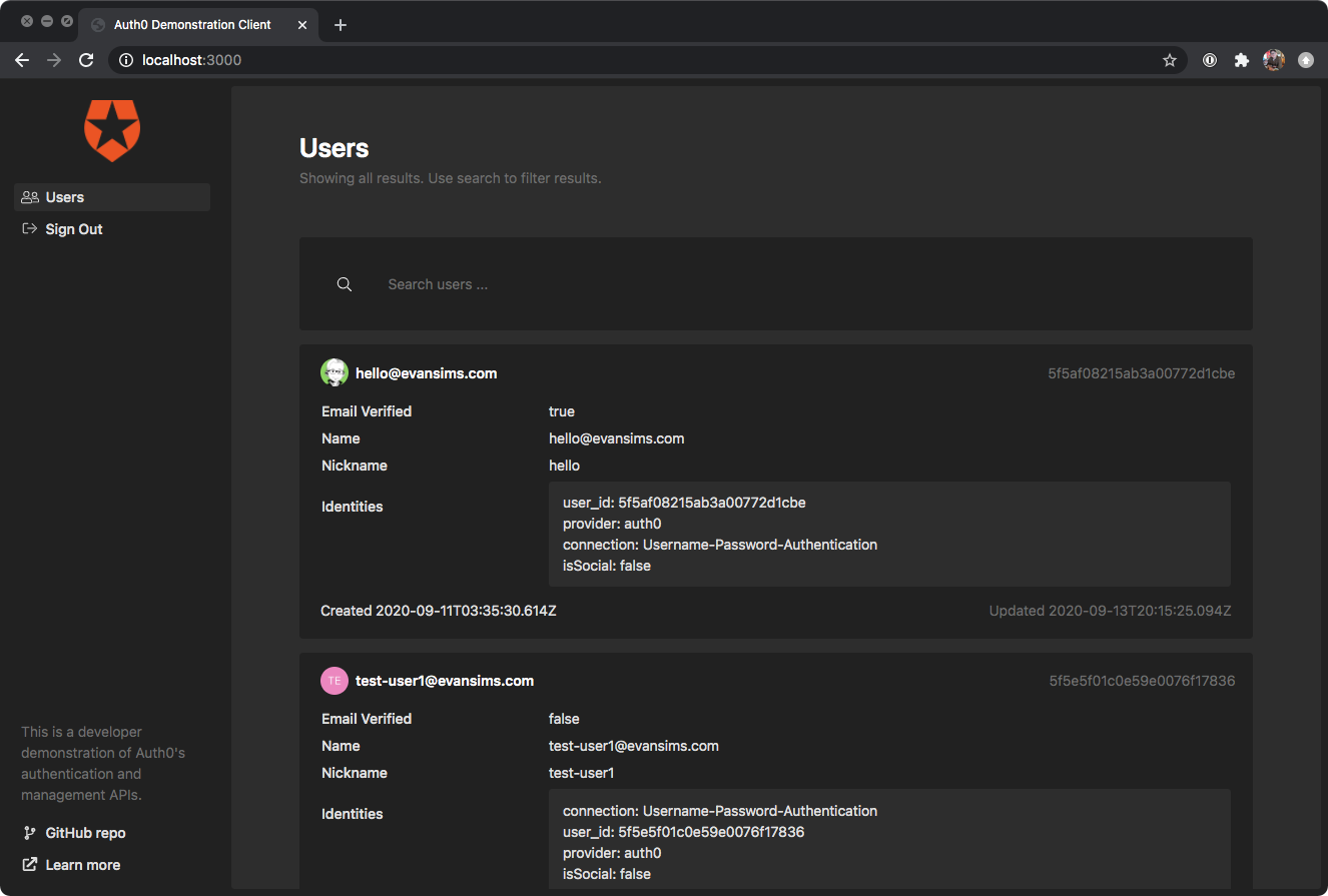
Thanks for your interest in my demonstration client of Auth0’s APIs. This is one half of a project demonstrating how one might go about implementing Auth0’s authentication API to interact with a custom backend.

This repository houses the JavaScript-based frontend server, using the Ember.js framework. The accompanying PHP-based backend server can be found here.

Requirements

Getting Started

You should begin by cloning and configuring the backend counterpart to this project first. Instructions for that can be found in it’s repository.

Next, clone this repository to your local machine:

git clone https://github.com/evansims/auth0-example-client.git

Quick Start Video Guide

Configure Auth0 application

Sign up for an Auth0 account, if you don’t already have one, and sign in.
Open Auth0’s Applications dashboard and create a new Single Page Web Application.
In your new Application’s settings, make note of your unique Client ID and Domain. You will need these later.
Set the ‘Allowed Callback URLs’ endpoint to http://localhost:3000/callback.
Save your Application settings changes.

Configure our client

On your machine, within the cloned directory of this repository, open the config/environment.js file.
Find the auth0 section.
Set your clientId and domain to the values you made note of when you set up your Auth0 Application (above.)
Set your audience to match the Audience of the Auth0 API you noted while configuring the backend server.
Save the file.

Build the client

This project assumes you have an existing Docker installation to simplify getting started. However, if you already have a working Ember CLI installation on your local machine you can build the project using the standard command line tools if you prefer.

We’ll be using docker-sync to help streamline the build process across platforms. Once you have docker-sync installed, open your shell to the cloned repository on your local machine and run:

$ docker-sync-stack start

This will begin a file sync to the Docker container and start the build process. This may take a few minutes to complete.

Once the build is done, your frontend will be accessible at http://localhost:3000 on your local machine.

To terminate the build process at any time, simply close the shell process, which on most platforms is usually accomplished by pressing CTRL+C.

Using the client

Open http://localhost:3000 on your local machine to use the client.

This client demonstrates a few simple aspects:

Authenticating users using Auth0’s SPA JS SDK with an Ember.js app
Communicating with a custom backend server to proxy calls to Auth0’s Management API, transforming our requests and enabling the following:
- Using Ember Data to store Auth0 user objects
- Rendering paginated results from the Management AP, using ember-concurrency
- Searching users with the Management API

After signing into the demonstration client with your Auth0 account, you will see a list of other users in your application.

You can paginate and view more users by selecting the ‘more users’ button at the bottom of the results.

At the top of the page you can use the search field to filter your results.

The important points

If you’re just looking for inspiration on how to do the important bits this client demonstrates, here’s where to look:

All session handling is done in the app/services/session.js file.
- The application route (app/routes/application.js) is the root route and always the first route called in an Ember app.
  - We use this opportunity to have Auth0’s SPA SDK check if the user has already authenticated. This automatically happens when we create the Auth0Client instance in our Session service’s getSession method.
- We have a method for getting some basic information about the authenticated user, getUser.
- We have a sign out method, releaseSession.
We have an Ember Data model representing all the user objects returned by the Management API at app/models/user.js
We use an Ember component for managing the calls to our custom backend and rendering the users at app/components/pages/accounts-list/component.js

Auth0 Documentation

Documentation for Auth0’s APIs can be found here.
Quickstarts for a variety of use cases, languages and respective frameworks can be found here.

Contributing

Pull requests are welcome!

Security Vulnerabilities

If you discover a security vulnerability within this project, please send an e-mail to Evan Sims at hello@evansims.com. All security vulnerabilities will be promptly addressed.

License

This demonstration project is open-sourced software licensed under the MIT license.

Simple Go Struct-Interface Method Example

Overview

This Go program demonstrates the use of interface-typed objects that are declared to link some functions to their specified struct. This technique, although using the property of interface-typed objects, is not the same as demonstrated here where interface-typed arguments are passed into functions. As for the code in this repository, we can use functions as methods for the created structs since we are not passing interface-typed objects as conventional argument, but we are using them as receiver arguments instead.

Program manual

Since this program is very similar to the one in the repository in this link, I’m just going to copy-paste the program manual from there as the following:

When run, the program asks the user to input the following information in the following order:

Note title
Note content
Todo
Then, the program will show messages containing the input information and, if there’s no error, will notify the user that the note and todo are successfully saved (in json file format).

There is no input validation for this program because every piece of information are in the form of free text. However, the program is designed to catch error when saving the files. The user will be notified if there’s any error while saving each file. In case of error, the program will stops after displaying the error message.

Code structure

Although, the program in this project works exactly the same as the one from this link, the code structure was designed differently in order to demonstrate another way of using interface to link common methods to different struct types from different packages.

The project comprises the main.go file which contains the code of the main program, and the codes which make up the note and todo packages. The main.go file contains the code declaring interface objects that link the save and display functions in the mentioned packages to their native structs. Those functions can, in turn, be used as the structs’ methods.

Program flow

Since this program works exactly as another one in a different repository as mentioned in several places above, I’m just going to copy an paste the same program flow from there as the following:

The user inputs the note title as a string
The user inputs the note content as a string
The program takes those inputs to create a struct which stores the note title, content, and the timestamp at its creation
The user inputs the todo text
The program takes the todo text input to create another struct which stores the todo text (without any title)
The program displays messages to confirm the note’s title and its content from the inputs
The program displays a message to confirm the todo
The program displays a message to notify the user that it’s saving the note
The program attempts to save the inputs as a json file with json field names according to the struct tags given in the code
The program displays the message that it saves the file successfully
The program repeat the same process from 8. for the todo (the todo’s file name is already hard-coded in the program and can’t be changed)

discord-uwu-bot

A Discord bot that translates regular text into UwU-speak.

Examples

English	UwU
Hello, world!	Hewlo, wowld! UwU!
Lorem ipsum dolar sit amet	Lowem ipsum dolaw sit amet UwU!
I’ll have you know I graduated top of my class in the Navy Seals	I’wl have you knyow I gwawduatewd top of my class in dwe Nyavy Seals UwU!

Commands

uwu*that – Uwuify a message in chat. Reply to a message to uwuifiy it.
uwu*this – Uwuify text. The rest of the message will be uwuified.
uwu*me – Follow the sender and translate everything that they say in the current channel.
uwu*stop [where] – Stop following the sender. Optionally set where to “channel”, “server”, or “everywhere” to stop following in the current channel, current server, or in all of Discord, respectively. Defaults to “channel”.
uwu*stop_everyone [where] – Stop following everyone in the current channel or server. Optionally set where to “channel” or “server” to specify where to stop following. Defaults to “channel”. Requires “Manage Messages” permission.
uwu*them <user> – Follow a specified user and translate everything that they say in the current channel. Requires “Manage Messages” permission. Use the command again to stop following.

Configuration

The bot can be configured through a JSON configuration file, located at /opt/UwuBot/appsettings.Production.json by default.
You must add your Discord token here before using the bot.
If you are using the the install script, then a default configuration file will be provided for you.
To create a configuration file manually, start with this template:

{
  "DiscordAuth": {
    "DiscordToken": "YOUR DISCORD TOKEN HERE",
  },
  "BotOptions": {
    "CommandPrefixes": [ "uwu*" ]
  },
  "UwuOptions": {
    "AppendUwu": true,
    "MakeCuteCurses": true
  }
}

The following options are available to customize the bot behavior:

Option	Description	Default
BotOptions:CommandPrefixes	List of command prefixes to respond to.	`[ "uwu*" ]`
UwuOptions:AppendUwu	Appends a trailing “UwU!” to the text.	`true`
UwuOptions:MakeCuteCurses	Replaces curse words with cuter, more UwU versions.	`true`

Discord Requirements (OAuth2)

To join the bot to a server, you must grant permissions integer 2048. This consists of:

bot scope
Send Messages permission

You must also grant the “Message Content” intent in the Discord Developer Portal.

System Requirements

.NET 6+
Windows, Linux, or MacOS. A version of Linux with SystemD (such as Ubuntu) is required to use the built-in install script and service definition.

Setup

Before you can run discord-uwu-bot, you need a Discord API Token.
You can get this token by creating and registering a bot at the Discord Developer Portal.
You can use any name or profile picture for your bot.
Once you have registered the bot, generate and save a Token.

Ubuntu / SystemD Linux

For Ubuntu (or other SystemD-based Linux systems), an install script and service definition are provided.
This install script will create a service account (default uwubot), a working directory (default /opt/UwuBot), and a SystemD service (default uwubot).
This script can update an existing installation and will preserve the appsettings.Production.json file containing your Discord Token and other configuration values.

Compile the bot or download pre-built binaries.
Run sudo ./install.sh.
[First install only] Edit /opt/UwuBot/appsettings.Production.json and add your Discord token.
Run sudo systemctl start uwubot to start the bot.

Other OS

For non-Ubuntu systems, manual setup is required.
The steps below are the bare minimum to run the bot, and do not include steps needed to create a persistent service.

Compile the bot or download pre-built binaries.
Edit appsettings.Production.json and add your Discord token.
Run dotnet DiscordUwuBot.Main.dll to start the bot.

What_I_Read

The book list what I read since 2017

2024

2023

2022

2021

2020

아주 작은 습관의 힘
그로스 해킹
오베라는 남자
Design patterns by tutorials
백종원의 장사 이야기
딥워크
연금술사
슈독
아몬드
세상을 만드는 글자, 코딩
셀트리오니즘

2019

홍콩산책
1시간에 1권 퀀텀 독서법
코딩을 지탱하는 기술
당신 거기 있어줄래요
한입에 웹 크롤링
수축사회
집 없이도 쉐어하우스로 제2의 월급 받는 사람들
블록체인 무엇인가
왜 세계의 절반은 굶주리는가
우리 이제 낭만을 이야기합시다
이십팔 독립선언
침대부터 정리하라
마케팅 천재가 된 맥스
Concurrency by Tutorials
손정의 300년 왕국의 야망
홍선표 기자의 써먹는 경제상식
타이탄
축구를 하며 생각한 것들
사업을 한다는 것
수상한 기록
Favorite magazine – We work together part1
50대 사건으로 보는 돈의 역사
꿈이 있으면 늙지 않는다
데미안
승려와 수수께끼

2018년

미중전쟁 2권
바깥은 여름
청춘의 돈 공부
옵션 B
서른의 반격
누워서 읽는 알고리즘
알고리즘 라이프
생각하는 늑대 타스케
편의점 인간
책 잘 읽는 방법
82년생 김지영
잠깐만 회사 좀 관두고 올게
거래의 기술
서른 살엔 미처 몰랐던 것들
바람이 되고 싶었던 아이
부자의 그릇
청년 기업가 정신
아마존, 세상의 모든 것을 팝니다
파괴적 혁신
문경수의 제주 과학 탐험
Favorite magazine – guest house

2017년

오리지널스
29살 생일 1년후 죽기로 결심했다
커피드림
나는 왜 정치를 하는가
스타트업 전성시대
고구려 4권
고구려 5권
소셜 코딩으로 이끄는 GitHub 실천기술
데드하트
예언
에어비앤비 스토리
남자의 물건
언어의 온도
명견만리(인구, 경제, 북한, 의료 편)
인공지능 투자가 퀀트
나미야 잡화점의 기적
미중전쟁 1권

Eclipse Paho JavaScript client

The Paho JavaScript Client is an MQTT browser-based client library written in Javascript that uses WebSockets to connect to an MQTT Broker.

Project description:

The Paho project has been created to provide reliable open-source implementations of open and standard messaging protocols aimed at new, existing, and emerging applications for Machine-to-Machine (M2M) and Internet of Things (IoT).
Paho reflects the inherent physical and cost constraints of device connectivity. Its objectives include effective levels of decoupling between devices and applications, designed to keep markets open and encourage the rapid growth of scalable Web and Enterprise middleware and applications.

Links

Project Website: https://www.eclipse.org/paho
Eclipse Project Information: https://projects.eclipse.org/projects/iot.paho
Paho Javascript Client Page: https://eclipse.org/paho/clients/js/
GitHub: https://github.com/eclipse/paho.mqtt.javascript
Twitter: @eclipsepaho
Issues: github.com/eclipse/paho.mqtt.javascript/issues
Mailing-list: https://dev.eclipse.org/mailman/listinfo/paho-dev

Using the Paho Javascript Client

Downloading

A zip file containing the full and a minified version the Javascript client can be downloaded from the Paho downloads page

Alternatively the Javascript client can be downloaded directly from the projects git repository: https://raw.githubusercontent.com/eclipse/paho.mqtt.javascript/master/src/paho-mqtt.js.

Please do not link directly to this url from your application.

Building from source

There are two active branches on the Paho Java git repository, master which is used to produce stable releases, and develop where active development is carried out. By default cloning the git repository will download the master branch, to build from develop make sure you switch to the remote branch: git checkout -b develop remotes/origin/develop

The project contains a maven based build that produces a minified version of the client, runs unit tests and generates it’s documentation.

To run the build:

$ mvn

The output of the build is copied to the target directory.

Tests

The client uses the Jasmine test framework. The tests for the client are in:

src/tests

To run the tests with maven, use the following command:

$ mvn test

The parameters passed in should be modified to match the broker instance being tested against.

Documentation

Reference documentation is online at: http://www.eclipse.org/paho/files/jsdoc/index.html

Compatibility

The client should work in any browser fully supporting WebSockets, http://caniuse.com/websockets lists browser compatibility.

Getting Started

The included code below is a very basic sample that connects to a server using WebSockets and subscribes to the topic World, once subscribed, it then publishes the message Hello to that topic. Any messages that come into the subscribed topic will be printed to the Javascript console.

This requires the use of a broker that supports WebSockets natively, or the use of a gateway that can forward between WebSockets and TCP.

// Create a client instance
var client = new Paho.MQTT.Client(location.hostname, Number(location.port), "clientId");

// set callback handlers
client.onConnectionLost = onConnectionLost;
client.onMessageArrived = onMessageArrived;

// connect the client
client.connect({onSuccess:onConnect});


// called when the client connects
function onConnect() {
  // Once a connection has been made, make a subscription and send a message.
  console.log("onConnect");
  client.subscribe("World");
  message = new Paho.MQTT.Message("Hello");
  message.destinationName = "World";
  client.send(message);
}

// called when the client loses its connection
function onConnectionLost(responseObject) {
  if (responseObject.errorCode !== 0) {
    console.log("onConnectionLost:"+responseObject.errorMessage);
  }
}

// called when a message arrives
function onMessageArrived(message) {
  console.log("onMessageArrived:"+message.payloadString);
}

Breaking Changes

Previously the Client’s Namepsace was Paho.MQTT, as of version 1.1.0 (develop branch) this has now been simplified to Paho.
You should be able to simply do a find and replace in your code to resolve this, for example all instances of Paho.MQTT.Client will now be Paho.Client and Paho.MQTT.Message will be Paho.Message.